Xanadu guide : https://github.com/golden75/prokaryote_RNASeq

This tutorial will serve as an introduction to analysis of prokaryote RNASeq data with an associated reference genome. The tools used for this analysis strictly consist of freeware and open-source software – any bioinformatician can perform the following analysis without any licenses!

Software download links:

SRA Toolkit
FastQC
Sickle
EDGE-pro
R
RStudio
DESeq2

RNASeq Workshop directory

/common/RNASeq_Workshop/Listeria

SRA Toolkit: Download raw reads in fastq format

The first step is to retrieve the biological sequence data from the Sequence Read Archive. The data that we will be using is from this experiment, which analyzes two strains of Listeria monocytogenes (10403S and DsigB) with two replicates per strain, resulting in a total of four raw read files. We will use the fastq-dump utility from the SRA toolkit to download the raw files by accession number into fastq format. This format is necessary because the software used to perform quality control, Sickle, requires fastq files as input.

module load sratoolkit/2.8.1
fastq-dump SRR034450
# repeat for SRR034451, SRR034452, SRR034453

The converted reads are located in the /common/RNASeq_Workshop/Listeria/Quality_Control/ directory. The script to convert the reads is located at: /common/RNASeq_Workshop/Listeria/Quality_Control/SRA_to_fastq.sh. Please note that this directory is write protected, meaning that the script will need to be run from a different directory. This is also the case for all scripts referenced throughout this tutorial – copy the scripts to a different directory before running them!

Since the fastqdump operation can be resource intensive, we will be submitting this script as a job to the cluster. Before doing so, replace the email in the line: #$ -M firstname.lastname@uconn.edu with your own email. Then submit the script with the qsub command:

qsub SRA-to-fastq.sh

For more information on using the BBC cluster and interacting with SGE please refer to this tutorial: http://bioinformatics.uconn.edu/understanding-the-bbc-cluster-and-sge/

FastQC

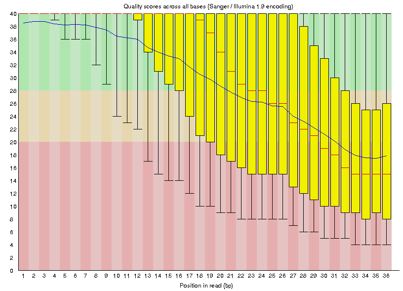
FastQC can be used to give an impression of the quality of the data before any further analysis such as quality control. We will run FastQC over the command line on just one of the .fastq files for demonstration purposes.

fastqc SRR034450.fastq

Once the program finishes running, the output will include an html formatted statistics file with the name SRR034450_fastqc.html. Copy this file to your desktop and open it with a web browser to view the contents, which will contain summary graphs and data such as the ‘Per base sequence quality graph’ below. 

Sickle: Quality Control on raw reads

The next step is to perform quality control on the reads using sickle. Since our reads are all unpaired reads, we indicate this with the se option in the sickle command. The -f flag designates the input file, -o the output file, and if desired -q the minimum quality (sickle defaults to 20) and -l the minimum read length. The -t flag designates the type of read. Unfortunately, despite the reads being Illumina reads, the average quality did not meet sickle’s minimum for Illumina reads, hence the sanger option.

sickle se -f SRR034450.fastq -t sanger -o SRR034450_trimmed.fastq
# repeat for SRR034451.fastq, SRR034452.fastq, SRR034453.fastq

The trimmed quality control fastq files are located in the /common/RNASeq_Workshop/Listeria/EDGE-pro directory. The files were moved there after running sickle for organization purposes — EDGE-pro requires the trimmed files as input. The script to perform the quality control is located at /common/RNASeq_Workshop/Listeria/Quality_Control/sickle_QC.sh.

EDGE-pro: Gene expression

Before we get started with EDGE-pro, we need to retrieve the Listeria reference genome and its protein and rna tables. By searching the NCBI genome database, we learn that the EGD-e strain is the reference genome. We will use NCBI’s ftp website: ftp://ftp.ncbi.nih.gov/ to download the files. Since Listeria is a bacterial genome, navigate to the genome directory then bacteria directory. Note that there are multiple genomes for Listeria — navigate to the EGD-e assembly: ftp://ftp.ncbi.nih.gov/genomes/Bacteria/Listeria_monocytogenes_EGD_e_uid61583/

The reference genome is stored in the .fna file, protein table in the .ptt file, and rna table in the .rnt file. We will use the wget command line utility to download these files.

wget http://genome2d.molgenrug.nl/Bacteria/Listeria_monocytogenes_EGD_e_uid61583/NC_003210.fna
wget http://genome2d.molgenrug.nl/Bacteria/Listeria_monocytogenes_EGD_e_uid61583/NC_003210.ptt
wget http://genome2d.molgenrug.nl/Bacteria/Listeria_monocytogenes_EGD_e_uid61583/NC_003210.rnt

Now we can run EDGE-pro to generate gene expression levels. The -g option takes a reference genome, -p flag a protein table, -r flag an rnt table, -u flag a fastq file (the trimmed file from sickle). The -o flag will be the prefix before each of the EDGE-pro output files, and the -s flag is the directory where the EDGE-pro executables are located.

/opt/bioinformatics/EDGE_pro_v1.3.1/edge.pl -g NC_003210.fna -p NC_003210.ptt -r NC_003210.rnt -u SRR034450_trimmed.fastq -o SRR034450.out -s /opt/bioinformatics/EDGE_pro_v1.3.1
# repeat for SRR034451_trimmed.fastq, SRR034452_trimmed.fastq, SRR034453_trimmed.fastq

The output files are located in the /common/RNASeq_Workshop/Listeria/EDGE-pro directory. The script to run EDGE-pro is located at /common/RNASeq_Workshop/Listeria/EDGE-pro/EDGE-pro.sh

EDGE-pro to DESeq

The output we are interested in are the SRR03445X.out.rpkm_0 files. EDGE-pro comes with an accessory script to convert the rpkm files to a count table that DESeq2, the differential expression analysis R package, can take as input.

/opt/bioinformatics/EDGE_pro_v1.3.1/additionalScripts/edgeToDeseq.perl SRR034450.out.rpkm_0 SRR034451.out.rpkm_0 SRR034452.out.rpkm_0 SRR034453.out.rpkm_0

Please note that EDGE-pro may sometimes create a second row for a gene with different count data than the first row. For our analysis with DESeq we desire each of the rows to be labeled with a gene ID, and this means that the list of genes must be unique. A python script was written to remove the duplicate row with the smallest total count. Writing this script is beyond the scope of this tutorial, but if you are interested, the script with comments is located at /common/RNASeq_Workshop/Listeria/EDGE-pro_to_DESeq2/trim_epro2deseq.py. This python script is executable globally so that you do not need to copy it to your own directory.  We will run the script as:

python /common/RNASeq_Workshop/Listeria/EDGE-pro_to_DESeq2/trim_epro2deseq.py deseqFile

where deseqFile is the intermediate output from edgeToDeseq.perl. The final, trimmed output table (a tab delimited file) is located at /common/RNASeq_Workshop/Listeria/EDGE-pro_to_DESeq2/Listeria_deseqFile. The script to generate the file is located at /common/RNASeq_Workshop/Listeria/EDGE-pro_to_DESeq2/to_DESeq2.sh and contains the commands to generate both the deseqFile and final Listeria_deseqFile.

Analysis with DESeq

This step requires the R language and an IDE such as RStudio installed on a local machine. The R DESeq2 library also must be installed. To install this package, start the R console and enter:

source("http://bioconductor.org/biocLite.R")
biocLite("DESeq2")

If any dependencies fail, install them using the command: install.packages(PackageName, repos='http://cran.rstudio.com/')

Before running this script make sure to set the working directory and path to your Listeria_deseqFile (after copying it from the server to your local machine). The script was adapted slightly from Dave Wheeler’s comprehensive tutorial on analysis with DESeq2 located here. The only changes were a few bug fixes, adding an outputPrefix variable to allow easy modification of the output file names in the code for future use, and adding filtering by adjusted p value.

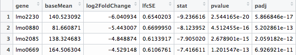
The most important information comes out as -replaceoutliers-results.csv. This file only contains the genes that have adjusted p values less than 0.05. These genes are the differentially expressed genes we are interested in. Depending on the experiment, this file can be adjusted to include p values less than 0.10 or a different value.

# Load DESeq2 library
library("DESeq2")

# Set the working directory
directory <- "~/Documents/R/DESeq2/"
setwd(directory)

# Set the prefix for each output file name
outputPrefix <- "Listeria_DESeq2"

# Location of deseq ready count table (EDGE-pro output)
deseqFile <- "~/Documents/R/DESeq2/Listeria_deseqFile"

# Read the table
countData <- read.table(deseqFile, header = T)

# Replace accession numbers with meaningful names
names(countData) <- c("10403S Rep1","DsigB Rep1","10403S Rep2","DsigB Rep2")

# Create table with treatment information
sampleNames <- colnames(countData)
sampleCondition <- c("10403S","DsigB","10403S","DsigB")
colData <- data.frame(condition = sampleCondition)
row.names(colData) = sampleNames
treatments = c("10403S","DsigB")

# Create DESeqDataSet: countData is the count table, colData is the table with treatment information
# One experimental condition
ddsFromMatrix <- DESeqDataSetFromMatrix(countData = countData,
 colData = colData,
 design = ~ condition)
colData(ddsFromMatrix)$condition <- factor(colData(ddsFromMatrix)$condition, levels = treatments)
dds <- DESeq(ddsFromMatrix)
res <- results(dds)

# filter results by p value
# order results by padj value (most significant to least)
res= subset(res, padj<0.05)
res <- res[order(res$padj),]
# should see DataFrame of baseMean, log2Foldchange, stat, pval, padj

# save data results and normalized reads to csv
resdata <- merge(as.data.frame(res), as.data.frame(counts(dds,normalized =TRUE)), by = 'row.names', sort = FALSE)
names(resdata)[1] <- 'gene'
write.csv(resdata, file = paste0(outputPrefix, "-results-with-normalized.csv"))

# send normalized counts to tab delimited file for GSEA, etc.
write.table(as.data.frame(counts(dds),normalized=T), file = paste0(outputPrefix, "_normalized_counts.txt"), sep = '\t')

# produce DataFrame of results of statistical tests
mcols(res, use.names = T)
write.csv(as.data.frame(mcols(res, use.name = T)),file = paste0(outputPrefix, "-test-conditions.csv"))

# replacing outlier value with estimated value as predicted by distrubution using
# "trimmed mean" approach. recommended if you have several replicates per treatment
# DESeq2 will automatically do this if you have 7 or more replicates
ddsClean <- replaceOutliersWithTrimmedMean(dds)
ddsClean <- DESeq(ddsClean)
tab <- table(initial = results(dds)$padj < 0.05,
 cleaned = results(ddsClean)$padj < 0.05)
addmargins(tab)
write.csv(as.data.frame(tab),file = paste0(outputPrefix, "-replaceoutliers.csv"))
resClean <- results(ddsClean)

# filter results by p value
resClean = subset(res, padj<0.05)
resClean <- resClean[order(resClean$padj),]
write.csv(as.data.frame(resClean),file = paste0(outputPrefix, "-replaceoutliers-results.csv"))

Here’s how your results file should look:

####################################################################################
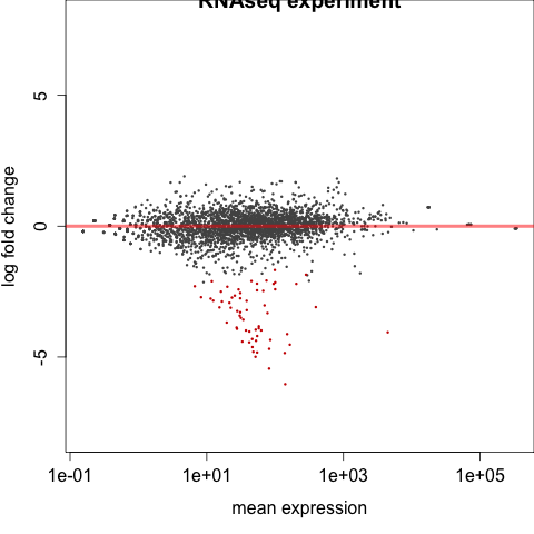
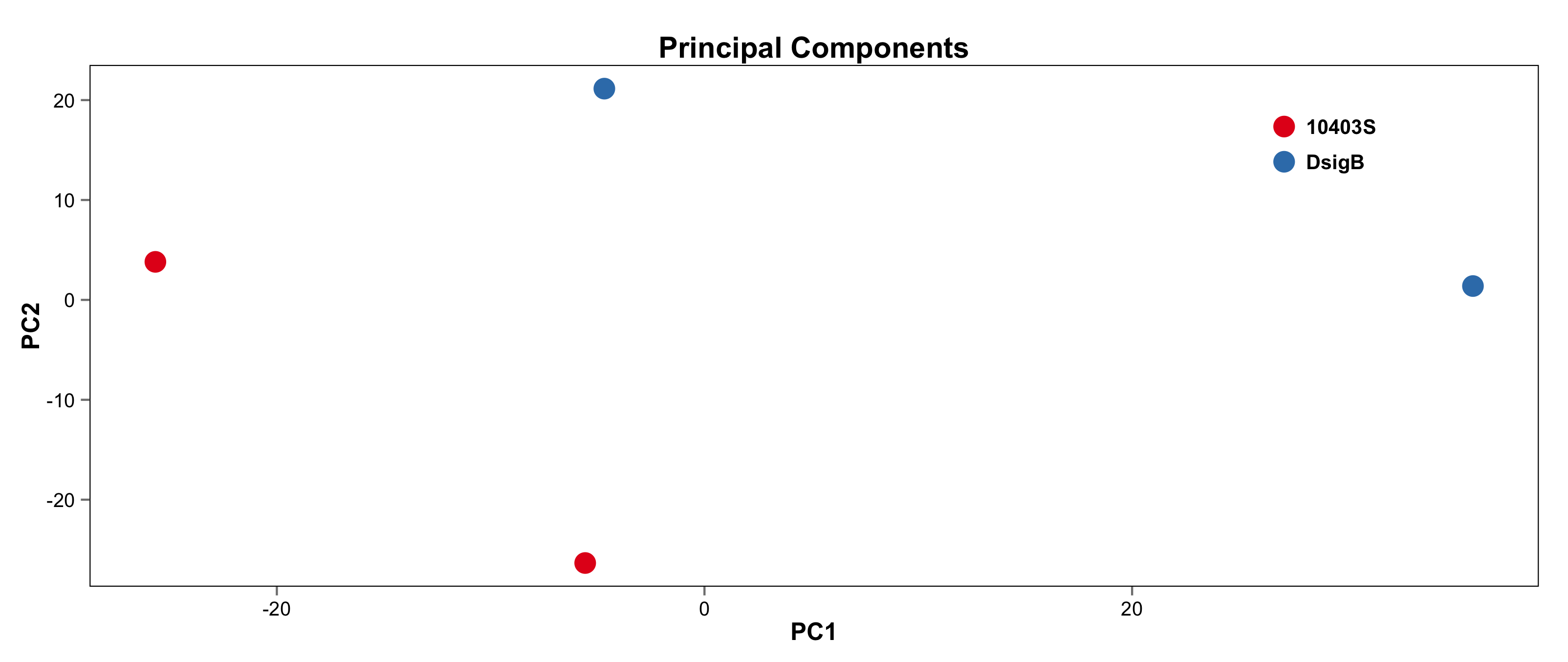
# Exploritory data analysis of RNAseq data with DESeq2
#
# these next R scripts are for a variety of visualization, QC and other plots to
# get a sense of what the RNAseq data looks like based on DESEq2 analysis
#
# 1) MA plot
# 2) rlog stabilization and variance stabiliazation
# 3) variance stabilization plot
# 4) heatmap of clustering analysis
# 5) PCA plot
#
#
####################################################################################
# MA plot of RNAseq data for entire dataset
# http://en.wikipedia.org/wiki/MA_plot
# genes with padj < 0.1 are colored Red
plotMA(dds, ylim=c(-8,8),main = "RNAseq experiment")
dev.copy(png, paste0(outputPrefix, "-MAplot_initial_analysis.png"))
dev.off()

# transform raw counts into normalized values
# DESeq2 has two options: 1) rlog transformed and 2) variance stabilization
# variance stabilization is very good for heatmaps, etc.
rld <- rlogTransformation(dds, blind=T)
vsd <- varianceStabilizingTransformation(dds, blind=T)

# save normalized values
write.csv(as.data.frame(assay(rld)),file = paste0(outputPrefix, "-rlog-transformed-counts.txt"))
write.csv(as.data.frame(assay(vsd)),file = paste0(outputPrefix, "-vst-transformed-counts.txt"))
 
# plot to show effect of transformation
# axis is square root of variance over the mean for all samples
par(mai = ifelse(1:4 <= 2, par('mai'),0))
px <- counts(dds)[,1] / sizeFactors(dds)[1]
ord <- order(px)
ord <- ord[px[ord] < 150]
ord <- ord[seq(1,length(ord),length=50)]
last <- ord[length(ord)]
vstcol <- c('blue','black')
matplot(px[ord], cbind(assay(vsd)[,1], log2(px))[ord, ],type='l', lty = 1, col=vstcol, xlab = 'n', ylab = 'f(n)')
legend('bottomright',legend=c(expression('variance stabilizing transformation'), expression(log[2](n/s[1]))), fill=vstcol)
dev.copy(png,paste0(outputPrefix, "-variance_stabilizing.png"))
dev.off()

#Principal components plot shows clustering of samples
library("genefilter")
library("ggplot2")
library("grDevices")

rv <- rowVars(assay(rld))
select <- order(rv, decreasing=T)[seq_len(min(500,length(rv)))]
pc <- prcomp(t(assay(vsd)[select,]))

# set condition
condition <- treatments
scores <- data.frame(pc$x, condition)

(pcaplot <- ggplot(scores, aes(x = PC1, y = PC2, col = (factor(condition)))) 
+ geom_point(size = 5)
+ ggtitle("Principal Components")
+ scale_colour_brewer(name = " ", palette = "Set1")
+ theme(
 plot.title = element_text(face = 'bold'),
 legend.position = c(.85,.87),
 legend.key = element_rect(fill = 'NA'),
 legend.text = element_text(size = 10, face = "bold"),
 axis.text.y = element_text(colour = "Black"),
 axis.text.x = element_text(colour = "Black"),
 axis.title.x = element_text(face = "bold"),
 axis.title.y = element_text(face = 'bold'),
 panel.grid.major.x = element_blank(),
 panel.grid.major.y = element_blank(),
 panel.grid.minor.x = element_blank(),
 panel.grid.minor.y = element_blank(),
 panel.background = element_rect(color = 'black',fill = NA)
))

ggsave(pcaplot,file=paste0(outputPrefix, "-ggplot2.png"))

# scatter plot of rlog transformations between Sample conditions
# nice way to compare control and experimental samples
# uncomment plots depending on size of array
# head(assay(rld))
plot(log2(1+counts(dds,normalized=T)[,1:2]),col='black',pch=20,cex=0.3, main='Log2 transformed')
plot(assay(rld)[,1:2],col='#00000020',pch=20,cex=0.3, main = "rlog transformed")
plot(assay(rld)[,3:4],col='#00000020',pch=20,cex=0.3, main = "rlog transformed")

# heatmap of data
library("RColorBrewer")
library("gplots")
# 30 top expressed genes with heatmap.2
select <- order(rowMeans(counts(ddsClean,normalized=T)),decreasing=T)[1:30]
my_palette <- colorRampPalette(c("blue",'white','red'))(n=30)
heatmap.2(assay(vsd)[select,], col=my_palette,
 scale="row", key=T, keysize=1, symkey=T,
 density.info="none", trace="none",
 cexCol=0.6, labRow=F,
 main="TITLE")
dev.copy(png, paste0(outputPrefix, "-HEATMAP.png"))
dev.off()

Selected tutorial results:

 

The R script and program output is available in the /common/RNASeq_Workshop/Listeria/R_DESeq2_output directory.