Galaxy is an open source, web-based platform for data intensive biomedical research. This tutorial is modified from Reference-based RNA-seq data analysis tutorial on github. In this tutorial, we will use Galaxy to analyze RNA sequencing data using a reference genome and to identify exons that are regulated by Drosophila melanogaster gene. To achieve that objectives, we will go through:

• Pretreatments
• Mapping
• Analysis of the differential expression
• Inference of the differential exon usage

Pretreatments
The original data we use is available at NCBI Gene Expression Omnibus(GEO) under accession number GSE18508
To conduct a Differential expression analysis, we will look at 7 first samples:

• 3 treated samples with Drosophila melanogaster gene depletion: GSM461179, GSM461180, GSM461181
• 4 untreated samples: GSM461176, GSM461177, GSM461178, GSM461182

Each sample constitutes a separate biological replicate of the corresponding condition (treated or untreated). Moreover, two of the treated and two of the untreated samples are from a paired-end sequencing assay, while the remaining samples are from a single-end sequencing experiment.

We have extracted sequences from the Sequence Read Archive (SRA) files to build FASTQ files. All files are available on Zenodo First we need create a new history for this RNA-seq exercise. Detailed instruction is shown below:

1. Click “History Option"icon on the top of History section.
2. Hit “create new”. A new history will be created. You may rename the name by directly editing it.

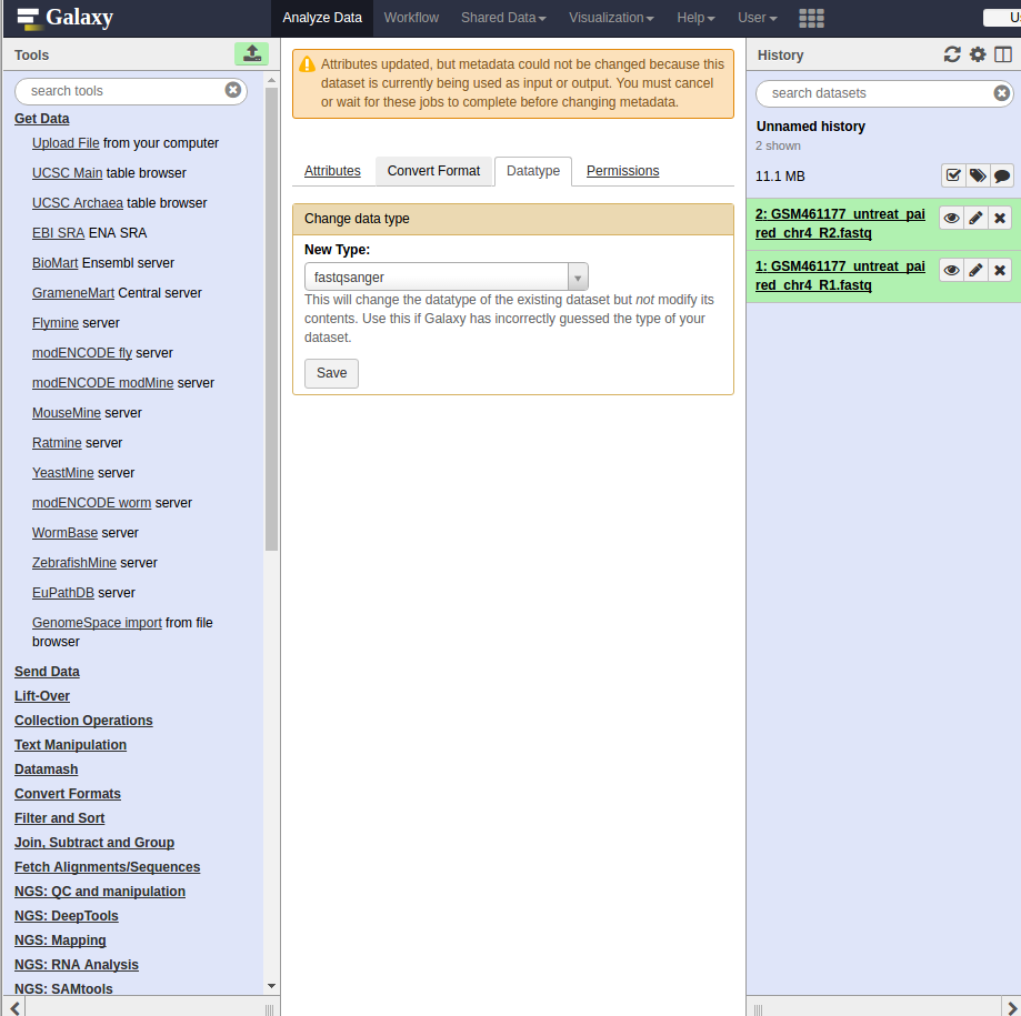
Then we need to import a FASTQ pair (e.g. GSM461177_untreat_paired_chr4_R1.fastq and GSM461177_untreat_paired_chr4_R2.fastq) from Zenodo, and convert file format to fastqsanger. Detailed instruction is shown below:

1. Copy the link location
2. Open the Galaxy Upload Manager
3. Select “Paste/Fetch Data”
4. Paste the link into the text field
5. Press Start (Note that Galaxy takes the link as name. It also do not link the dataset to a database or a reference genome as default)
6. Click on the pencil button displayed in your dataset in the history
7. Rename the datasets according to the samples
8. Press Save
9. Choose Datatype on the top
10. Select fastqsanger
11. Press Save

Both files contain the reads that belong to chromosome 4 of a paired-end sample. The sequences are raw sequences from the sequencing machine, without any pretreatments. They need to be controlled for their quality.

For quality control, we use FastQC and Trim Galore. We first run Fastqc on both FastQ files to check quality of reads.

1. Select the paired ended dataset (e.g GSM461177_untreat_paired_chr4_R1.fastq and GSM461177_untreat_paired_chr4_R2.fastq)
2. Find and open FastQC from Tools bar
3. Press Execute

Then treat for the quality of sequences by running Trim Galore on the paired-end datasets.

1. Find and open FastQC from Tools
2. Choose  “Pair-end”
3. Use default value for other parameters
4. Select the paired ended dataset
5. Press “Execute”

Finally, we may re-run FastQC on Trim Galore’s outputs and inspect the differences.

 

Mapping
To make sense of the reads, their positions within Drosophila melanogaster genome must be determined. This process is known as aligning or ‘mapping’ the reads to the reference genome. Here, we will use HISAT2, a successor to TopHat2 that is faster with low memory requirements.To run efficiently the mapping, HISAT2 needs to know on important parameters about the sequencing library: the library type. This information should usually come with your FASTQ files, ask your sequencing facility! If not, try to find them on the site where you downloaded the data or in the corresponding publication. Another option is to estimate these parameters with a preliminary mapping of a downsampled file and some analysis programs. Afterward, the actual mapping can be redone on the original files with the optimized parameters.

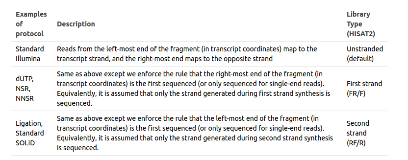
We first need to run a preliminary mapping, we will estimate the library type to run HISAT2 efficiently afterwards. This step is not necessary if you don’t need to estimate the library type of your data. The library type corresponds to a protocol used to generate the data: which strand the RNA fragment is synthesized from.

In the previous illustration, you could see that for example dUTP method is to only sequence the strand from the first strand synthesis (the original RNA strand is degradated due to the dUTP incorporated).

If you do not know the library type, you can find it by yourself by mapping the reads on the reference genome and infer the library type from the mapping results by comparing reads mapping information to the annotation of the reference genome.

The sequencer always read from 5’ to 3’. So, in First Strand case, all reads from the left-most end of RNA fragment (always from 5’ to 3’) are mapped to transcript-strand, and (for pair-end sequencing) reads from the right-most end are always mapped to the opposite strand.

We can now try to determine the library type of our data. The first step is loading the Ensembl gene annotation for Drosophila melanogaster (Drosophila_melanogaster.BDGP5.78.gtf) from Zenodo into your current Galaxy history and rename it.

Next, we run HISAT2 with:

1. “FASTQ” as “Input data format”
2. “Individual paired reads”
3. Downsampled “Trimmed reads pair 1” (Trim Galore output) as “Forward reads”
4. Downsampled “Trimmed reads pair 2” (Trim Galore output) as “Reverse reads”
5. “dm3” as reference genome
6. Default values for other parameters

Then run Infer Experiment to determine the library type:

1. 1. HISAT2 output as “Input BAM/SAM file”
   2. Drosophila annotation as “Reference gene model”

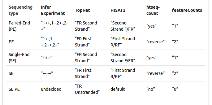
Sometimes it is difficult to find out which settings correspond to those of other programs. The following table might be helpful to identify library type:

We can now map all the RNA sequences on the Drosophila melanogaster genome using HISAT2. HISAT2 will output a BAM file.

1. 1. 1. FASTQ” as “Input data format”
      2. “Individual paired reads”
      3. “Trimmed reads pair 1” (Trim Galore output) as “Forward reads”
      4. “Trimmed reads pair 2” (Trim Galore output) as “Reverse reads”
      5. “dm3” as reference genome
      6. Default values for other parameters except “Spliced alignment parameters”
      7. “Specify strand-specific information” to the previously determined value
      8. Drosophila_melanogaster.BDGP5.78.gtf as “GTF file with known splice sites”

We can inspect the mapping statistics:

1. 1. 1. Click on “View details” (Warning icon)
      2. Click on “stderr” (Tool Standard Error)

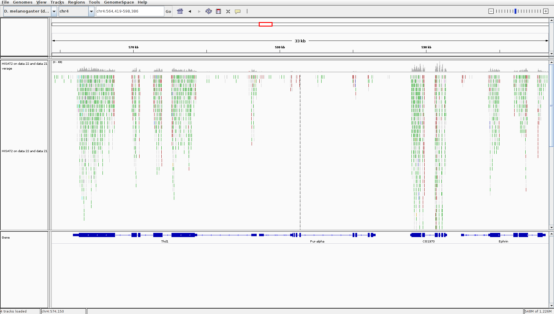
The BAM file contains information about where the reads are mapped on the reference genome. But it is binary file and with the information for more than 3 millions of reads, it makes it difficult to visualize it. We use IGV to visualize the HISAT2 output BAM file, particularly the region on chromosome 4 between 560kb to 600 kb.

1. Download and install IGV on your local machine by following instruction found here
2. Hit the BAM file
3. click “local” under display with IGV

Analysis of the differential gene expression
To compare the expression of single genes between different conditions (e.g. with or without PS depletion), an first essential step is to quantify the number of reads per gene. HTSeq-count is one of the most popular tool for gene quantification.To quantify the number of reads mapped to a gene, an annotation of the gene position is needed. We already upload on Galaxy the <code>Drosophila_melanogaster.BDGP5.78.gtf</code> with the Ensembl gene annotation for Drosophila melanogaster.

In principle, the counting of reads overlapping with genomic features is a fairly simple task. But there are some details that need to be decided, such how to handle multi-mapping reads. HTSeq-count offers 3 choices (“union”, “intersection_strict” and “intersection_nonempty”) to handle read mapping to multiple locations, reads overlapping introns, or reads that overlap more than one genomic feature:

The recommended mode is “union”, which counts overlaps even if a read only shares parts of its sequence with a genomic feature and disregards reads that overlap more than one feature.

1. Drosophila_melanogaster.BDGP5.78.gtf as “GFF file”
2. The “Union” mode
3. A “Minimum alignment quality” of 10
4. Appropriate value for “Stranded” option

For time and computer saving, in this section, we run the previous steps for you and obtain 7 count files, available on Zenodo. These files contain for each gene of Drosophila the number of reads mapped to it. We could compare directly the files and then having the differential gene expression. But the number of sequenced reads mapped to a gene depends on some other factors, such as expression level, length,and sequencing depth. Either for within or for inter-sample comparison, the gene counts need to be normalized. We can then use the Differential Gene Expression (DGE) analysis. This expression analysis is estimated from read counts and attempts are made to correct for variability in measurements using replicates that are absolutely essential accurate results. For your own analysis, we advice you to use at least 3, better 5 biological replicates per condition. You can have different number of replicates per condition. In our example, there are 2 factors that can explain differences in gene expression, treatment and sequencing type. Here treatment is the primary factor which we are interested in.

DESeq2 is a great tool for DGE analysis. It takes read counts produced by HTseq-count, combine them into a big table (with gene in the rows and samples in the columns) and applies size factor normalization. To import read count files and run DESeq2, follow instruction shown below:

1. Create a new history
2. import the seven count files from Zenodo
3. Run DESeq2
4. Set “Treatment” as first factor with “treated”
   and “untreated” as levels and selection of count files corresponding to both levels
5. Press “insert factor”
6. set “Sequencing” as second factor with “PE” and “SE” as levels and selection of count files corresponding to both levels (Keeping the CTRL key pressed and clicking on the files to select several files)
7. hit “execute”

The first output of DESeq2 is a tabular file. The columns are:

• Gene identifiers
• Mean normalized counts, averaged over all samples from both conditions
• Logarithm (to basis 2) of the fold change
• Standard error estimate for the log2 fold change estimate
• Wald statistic
• p-value for the statistical significance of this change
• p-value adjusted for multiple testing with the Benjamini-Hochberg procedure which controls false discovery rate (FDR)

To extract genes with most significant changes (adjusted p-value equal or below 0.05), we use Filter.

1. Launch Filter
2. Select the DESeq2 result table as input
3. Type c7 < 0.05 in “With following condition”
4. Press “execute”
5. (optional)rename the output file for downstream analysis

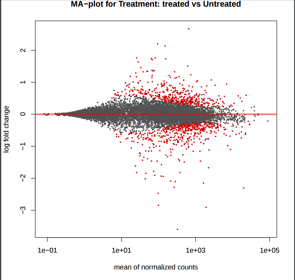
In addition to the list of genes, DESeq2 outputs a graphical summary of the results, useful to evaluate the quality of the experiment based on histogram of p-values for all tests, MA plot, principal Component Analysis (PCA), Heatmap of sample-to-sample distance matrix, and dispersion estimate.

MA plot provides a global view of the relationship between the expression change of conditions (log ratios, M), the average expression strength of the genes (average mean, A), and the ability of the algorithm to detect differential gene expression. The genes that passed the significance threshold (adjusted p-value < 0.25) are colored in red.

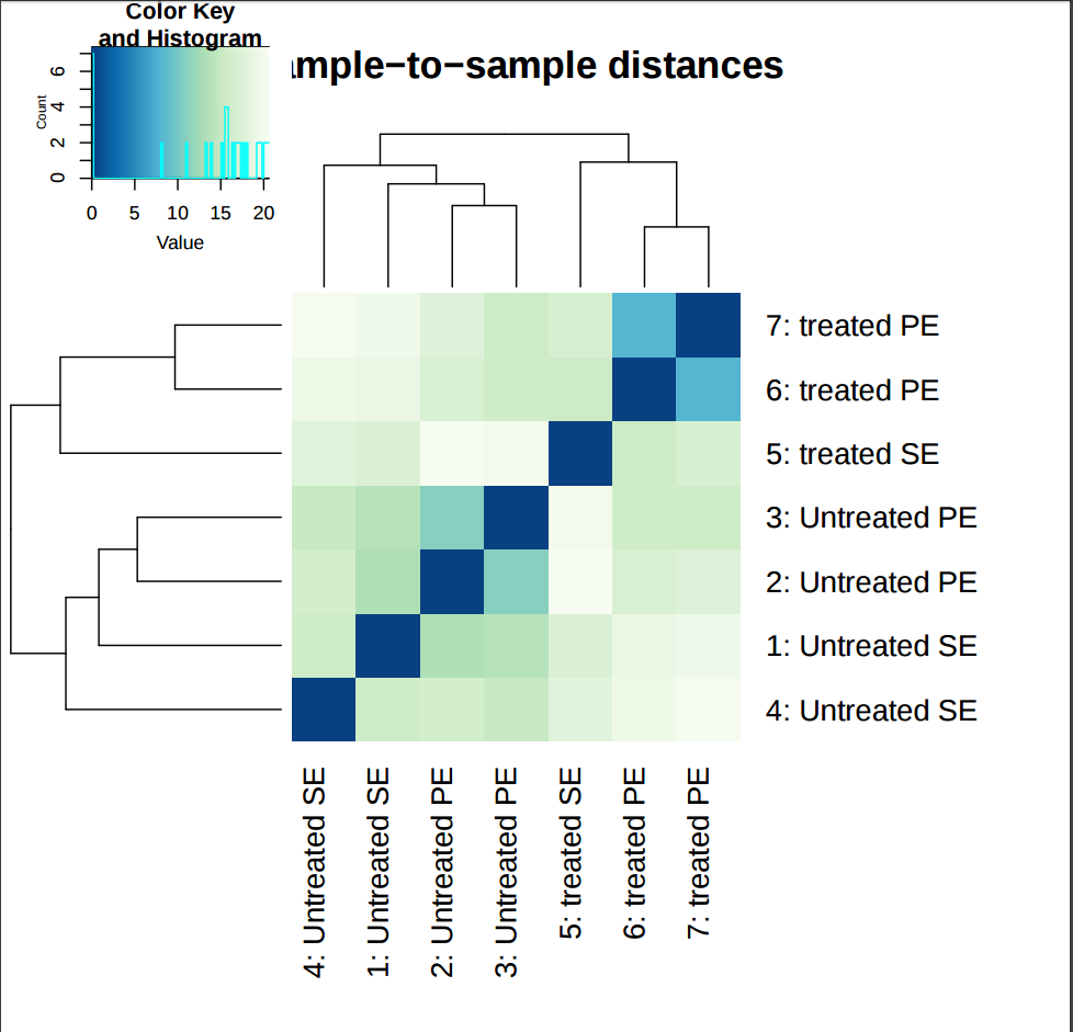
The heatmap provides overview over similarities and dissimilarities between samples.

Dispersion estimates: gene-wise estimates (black), the fitted values (red), and the final maximum a posteriori estimates used in testing (blue)

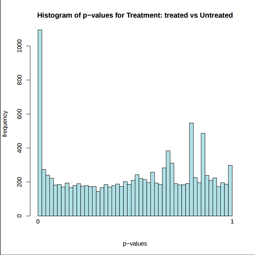
Histogram of p-values:

Analysis of the functional enrichment among differentially expressed genes

We have extracted genes that are differentially expressed in treated (with PS gene depletion) samples compared to untreated samples. We would like to know the functional enrichment among the differentially expressed genes.

The Database for Annotation, Visualization and Integrated Discovery (DAVID) provides a comprehensive set of functional annotation tools for investigators to understand the biological meaning behind large lists of genes.

The query to DAVID can be done only on 100 genes. So, we will need to select the ones where the most interested in.

1. Launch Sort tool
2. Select previously filtered file under “Sort Query”
3. “Column:3” under “on column” and “Descending order under “everything in” to check most unregulated genes
4. Press “Execute”
5. Launch Select first tool
6. Extract first 100 lines
7. Lauch DAVID
8. First column as “Column with identifiers”
9. “ENSEMBL_GENE_ID” as “Identifier type”
10. press “Execute”

The output of the DAVID tool is a HTML file with a link to the DAVID website.

Inference of the differential exon usage
Now, we would like to know the differential exon usage between treated (PS depleted) and untreated samples using RNA-seq exon counts. We will rework on the mapping results we generated previously.

We will use DEXSeq. DEXSeq detects high sensitivity genes, and in many cases exons, that are subject to differential exon usage. But first, as for the differential gene expression, we need to count the number of reads mapping the exons.

Similar to the step of counting the number of reads per annotated gene. Here instead of HTSeq-count, we are using DEXSeq-Count

1. Transfer Gene annotation file Drosophila_melanogaster.BDGP5.78.gtf from Zenodo to a Galaxy history.
2. Launch “DEXSeq-Count”
3. “Prepare annotation” of “Mode of operation”

The output is again a GTF file that is ready to be used for counting. To count reads using DEXSeq-Count,

1. “count reads” as “Mode of operation”
2. “HISAT2 output as “Input bam file”
3. GTF file from previous step as “DEXSeq compatible GTF file”

This output a flatten GTF file.

Next, we calculate differential exon usage. As for DESeq2, in the previous step, we counted only reads that mapped to exons on chromosome 4 and for only one sample. To be able to identify differential exon usage induced by PS depletion, all datasets (3 treated and 4 untreated) must be analyzed with the similar procedure. For time saving, we use results available on Zenodo.

1. Create a new history
2. Import the seven count files from Zenodo and the gtf file generated from previous step
3. Launch DEXSeq
4. “Condition” as first factor with “treated” and “untreated” as levels and selection of count files corresponding to both levels
5. “Sequencing” as second factor with “PE” and “SE” as levels and selection of count files corresponding to both levels

Note that unlike DESeq2, DEXSeq does not allow flexible primary factor names. Always use your primary factor name as “condition”. This step will take a couple hours to run.

Similarly to DESeq2, DEXSeq generates a table with:

• Exon identifiers
• Gene identifiers
• Exon identifiers in the Gene
• Mean normalized counts, averaged over all samples from both conditions
• Logarithm (to basis 2) of the fold change
• Standard error estimate for the log2 fold change estimate
• p-value for the statistical significance of this change
• p-value adjusted for multiple testing with the Benjamini-Hochberg procedure which controls false discovery rate

Similarly, we also run Filter to extract exons with a a significant usage (adjusted p-value equal or below 0.05) between treated and untreated samples.

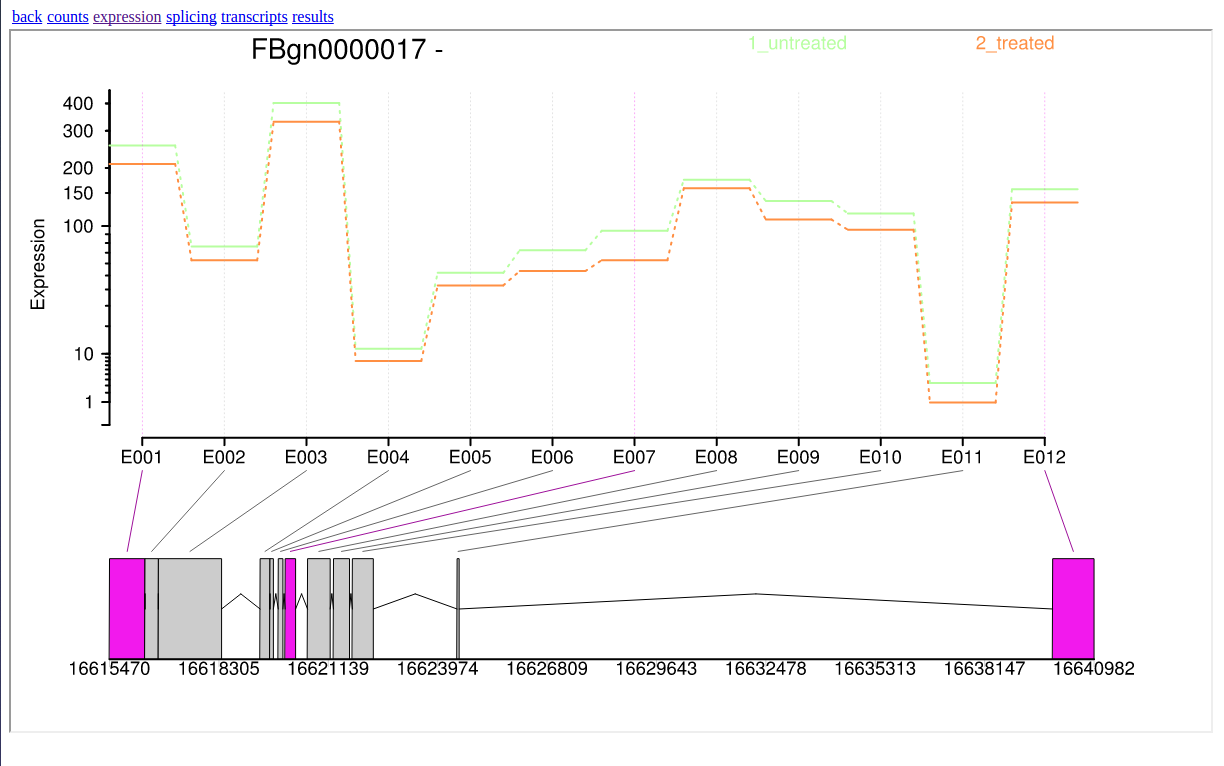
In addition, DEXSeq generates a interactive HTML file which allows users to inspect deferentially expressed exons graphically.

In this tutorial, we have analyzed real RNA sequencing data to extract useful information, such as which genes are up- or downregulated by depletion of the Drosophila melanogaster gene and which genes are regulated by the Drosophila melanogaster gene. To answer these questions, we analyzed RNA sequence datasets using a reference-based RNA-seq data analysis approach. This approach can be sum up with the following scheme: