This tutorial will serve as a guideline for how to go about analyzing RNA sequencing data when a reference genome is available. We will be going through quality control of the reads, alignment of the reads to the reference genome, conversion of the files to raw counts, analysis of the counts with DeSeq2, and finally annotation of the reads using Biomart. Most of this will be done on the BBC server unless otherwise stated.
The packages we’ll be using can be found here: Page by Dister Deoss
The data we will be using are comparative transcriptomes of soybeans grown at either ambient or elevated O3 levels. Each condition was done in triplicate, giving us a total of six samples we will be working with. The paper that these samples come from (which also serves as a great background reading on RNA-seq) can be found here:
The Bench Scientist’s Guide to statistical Analysis of RNA-Seq Data
The samples we will be using are described by the following accession numbers; SRR391535, SRR391536, SRR391537, SRR391538, SRR391539, and SRR391541. They can be found in results 13 through 18 of the following NCBI search:
http://www.ncbi.nlm.nih.gov/sra/?term=SRP009826
The script for downloading these .SRA files and converting them to fastq can be found in
/common/RNASeq_Workshop/Soybean/Quality_Control as the file fastq-dump.sh. The fastq files themselves are also already saved to this same directory.
module load sratoolkit/2.8.1
fastq-dump SRR391535
Quality Control on the Reads Using Sickle:
Step one is to perform quality control on the reads using Sickle. We are using unpaired reads, as indicated by the “se” flag in the script below. The -f flag designates the input file, -o is the output file, -q is our minimum quality score and -l is the minimum read length. The trimmed output files are what we will be using for the next steps of our analysis.
sickle se -f SRR391535.fastq -t sanger -o trimmed_SRR391535.fastq -q 35 -l 45
The script for running quality control on all six of our samples can be found in
/common/RNASeq_Workshop/Soybean/Quality_Control as the file sickle_soybean.sh. The output trimmed fastq files are also stored in this directory.
Alignment of Trimmed Reads Using STAR:
For this next step, you will first need to download the reference genome and annotation file for Glycine max (soybean). The files I used can be found at the following link:
You will need to create a user name and password for this database before you download the files. Once you’ve done that, you can download the assembly file Gmax_275_v2 and the annotation file Gmax_275_Wm82.a2.v1.gene_exons. Having the correct files is important for annotating the genes with Biomart later on.
Now that you have the genome and annotation files, you will create a genome index using the following script:
STAR --runMode genomeGenerate --genomeDir /common/RNASeq_Workshop/Soybean/gmax_genome/ --genomeFastaFiles /common/RNASeq_Workshop/Soybean/gmax_genome/Gmax_275_v2 --sjdbGTFfile /common/RNASeq_Workshop/Soybean/gmax_genome/Gmax_275_Wm82.a2.v1.gene_exons --sjdbGTFtagExonParentTranscript Parent --sjdbOverhang 100 --runThreadN 8
You will likely have to alter this script slightly to reflect the directory that you are working in and the specific names you gave your files, but the general idea is there. Indexing the genome allows for more efficient mapping of the reads to the genome.
The assembly file, annotation file, as well as all of the files created from indexing the genome can be found in
/common/RNASeq_Workshop/Soybean/gmax_genome
Now that you have your genome indexed, you can begin mapping your trimmed reads with the following script:
STAR --genomeDir /common/RNASeq_Workshop/Soybean/gmax_genome/ --readFilesIn trimmed_SRR391535.fastq --runThreadN 8 --outSAMtype BAM SortedByCoordinate --outFileNamePrefix SRR391535
The –genomeDir flag refers to the directory in which your indexed genome is located. The output we get from this are .BAM files; binary files that will be converted to raw counts in our next step.
The script for mapping all six of our trimmed reads to .bam files can be found in
/common/RNASeq_Workshop/Soybean/STAR_HTSEQ_mapping as the file star_soybean.sh. The .bam output files are also stored in this directory.
Convert BAM Files to Raw Counts with HTSeq:
Finally, we will use HTSeq to transform these mapped reads into counts that we can analyze with R. “-s” indicates we do not have strand specific counts. “-r” indicates the order that the reads were generated, for us it was by alignment position. “-t” indicates the feature from the annotation file we will be using, which in our case will be exons. “-i” indicates what attribute we will be using from the annotation file, here it is the PAC transcript ID. We identify that we are pulling in a .bam file (“-f bam”) and proceed to identify, and say where it will go.
htseq-count -s no -r pos —t exon -i pacid -f bam SRR391535Aligned.sortedByCoord.out.bam /common/RNASeq_Workshop/Soybean/gmax_genome/Gmax_275_Wm82.a2.v1.gene_exons > SRR391535-output_basename.counts
The script for converting all six .bam files to .count files is located in
/common/RNASeq_Workshop/Soybean/STAR_HTSEQ_mapping as the file htseq_soybean.sh. The .count output files are saved in
/common/RNASeq_Workshop/Soybean/STAR_HTSEQ_mapping/counts
Analysis of Counts with DESeq2:
For the remaining steps I find it easier to to work from a desktop rather than the server. So you can download the .count files you just created from the server onto your computer. You will also need to download R to run DESeq2, and I’d also recommend installing RStudio, which provides a graphical interface that makes working with R scripts much easier. They can be found here:
The R DESeq2 library also must be installed. To install this package, start the R console and enter:
source("http://bioconductor.org/biocLite.R")
biocLite("DESeq2")
The R code below is long and slightly complicated, but I will highlight major points. This script was adapted from here and here, and much credit goes to those authors. Some important notes:
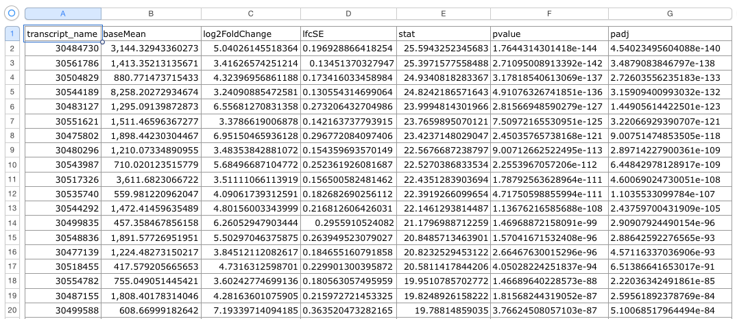
- The most important information comes out as “-replaceoutliers-results.csv” there we can see adjusted and normal p-values, as well as log2foldchange for all of the genes.
- par(mar) manipulation is used to make the most appealing figures, but these values are not the same for every display or system or figure. Much documentation is available online on how to manipulate and best use par() and ggplot2 graphing parameters: DESeq2 Manual
# Load DESeq2 library
library("DESeq2")
# Set the working directory
directory <- "~/Documents/counts2"
setwd(directory)

# Set the prefix for each output file name
outputPrefix <- "Gmax_DESeq2"

sampleFiles<- c("SRR391535-output_basename.counts",
                "SRR391536-output_basename.counts",
                "SRR391537-output_basename.counts",
                "SRR391538-output_basename.counts",
                "SRR391539-output_basename.counts",
                "SRR391541-output_basename.counts")
sampleNames <- c("Leaf tissue 1","Leaf tissue 2","Leaf tissue 3","Leaf tissue 4","Leaf tissue 5","Leaf tissue 6")
sampleCondition <- c("ambient","ambient","elevated","elevated","elevated","ambient")
sampleTable <- data.frame(sampleName = sampleNames, fileName = sampleFiles, condition = sampleCondition)

treatments = c("ambient","elevated")

library("DESeq2")
ddsHTSeq <- DESeqDataSetFromHTSeqCount(sampleTable = sampleTable,
                                       directory = directory,
                                       design = ~ condition)
colData(ddsHTSeq)$condition <- factor(colData(ddsHTSeq)$condition,
                                      levels = treatments)

#guts
dds <- DESeq(ddsHTSeq)
res <- results(dds)

# copied from: https://benchtobioinformatics.wordpress.com/category/dexseq/
# order results by padj value (most significant to least)
res= subset(res, padj<0.05)
res <- res[order(res$padj),]
# should see DataFrame of baseMean, log2Foldchange, stat, pval, padj

# save data results and normalized reads to csv
resdata <- merge(as.data.frame(res), as.data.frame(counts(dds,normalized =TRUE)), by = 'row.names', sort = FALSE)
names(resdata)[1] <- 'gene'
write.csv(resdata, file = paste0(outputPrefix, "-results-with-normalized.csv"))

# send normalized counts to tab delimited file for GSEA, etc.
write.table(as.data.frame(counts(dds),normalized=T), file = paste0(outputPrefix, "_normalized_counts.txt"), sep = '\t')

# produce DataFrame of results of statistical tests
mcols(res, use.names = T)
write.csv(as.data.frame(mcols(res, use.name = T)),file = paste0(outputPrefix, "-test-conditions.csv"))

# replacing outlier value with estimated value as predicted by distrubution using
# "trimmed mean" approach. recommended if you have several replicates per treatment
# DESeq2 will automatically do this if you have 7 or more replicates

ddsClean <- replaceOutliersWithTrimmedMean(dds)
ddsClean <- DESeq(ddsClean)
tab <- table(initial = results(dds)$padj < 0.05,
             cleaned = results(ddsClean)$padj < 0.05)
addmargins(tab)
write.csv(as.data.frame(tab),file = paste0(outputPrefix, "-replaceoutliers.csv"))
resClean <- results(ddsClean)
resClean = subset(res, padj<0.05)
resClean <- resClean[order(resClean$padj),]
write.csv(as.data.frame(resClean),file = paste0(outputPrefix, "-replaceoutliers-results.csv"))

####################################################################################
# Exploratory data analysis of RNAseq data with DESeq2
#
# these next R scripts are for a variety of visualization, QC and other plots to
# get a sense of what the RNAseq data looks like based on DESEq2 analysis
#
# 1) MA plot
# 2) rlog stabilization and variance stabiliazation
# 3) variance stabilization plot
# 4) heatmap of clustering analysis
# 5) PCA plot
#
#
####################################################################################

# MA plot of RNAseq data for entire dataset
# http://en.wikipedia.org/wiki/MA_plot
# genes with padj < 0.1 are colored Red
plotMA(dds, ylim=c(-8,8),main = "RNAseq experiment")
dev.copy(png, paste0(outputPrefix, "-MAplot_initial_analysis.png"))
dev.off()

# transform raw counts into normalized values
# DESeq2 has two options:  1) rlog transformed and 2) variance stabilization
# variance stabilization is very good for heatmaps, etc.
rld <- rlogTransformation(dds, blind=T)
vsd <- varianceStabilizingTransformation(dds, blind=T)

# save normalized values
write.table(as.data.frame(assay(rld),file = paste0(outputPrefix, "-rlog-transformed-counts.txt"), sep = '\t'))
write.table(as.data.frame(assay(vsd),file = paste0(outputPrefix, "-vst-transformed-counts.txt"), sep = '\t'))

# plot to show effect of transformation
# axis is square root of variance over the mean for all samples
par(mai = ifelse(1:4 <= 2, par('mai'),0))
px <- counts(dds)[,1] / sizeFactors(dds)[1]
ord <- order(px)
ord <- ord[px[ord] < 150]
ord <- ord[seq(1,length(ord),length=50)]
last <- ord[length(ord)]
vstcol <- c('blue','black')
matplot(px[ord], cbind(assay(vsd)[,1], log2(px))[ord, ],type='l', lty = 1, col=vstcol, xlab = 'n', ylab = 'f(n)')
legend('bottomright',legend=c(expression('variance stabilizing transformation'), expression(log[2](n/s[1]))), fill=vstcol)
dev.copy(png,paste0(outputPrefix, "-variance_stabilizing.png"))
dev.off()

# clustering analysis
# excerpts from http://dwheelerau.com/2014/02/17/how-to-use-deseq2-to-analyse-rnaseq-data/
library("RColorBrewer")
library("gplots")
distsRL <- dist(t(assay(rld)))
mat <- as.matrix(distsRL)
rownames(mat) <- colnames(mat) <- with(colData(dds), paste(condition, sampleNames, sep=" : "))
#Or if you want conditions use:
#rownames(mat) <- colnames(mat) <- with(colData(dds),condition)
hmcol <- colorRampPalette(brewer.pal(9, "GnBu"))(100)
dev.copy(png, paste0(outputPrefix, "-clustering.png"))
heatmap.2(mat, trace = "none", col = rev(hmcol), margin = c(13,13))
dev.off()

#Principal components plot shows additional but rough clustering of samples
library("genefilter")
library("ggplot2")
library("grDevices")

rv <- rowVars(assay(rld))
select <- order(rv, decreasing=T)[seq_len(min(500,length(rv)))]
pc <- prcomp(t(assay(vsd)[select,]))

# set condition
condition <- treatments
scores <- data.frame(pc$x, condition)

(pcaplot <- ggplot(scores, aes(x = PC1, y = PC2, col = (factor(condition))))
+ geom_point(size = 5)
+ ggtitle("Principal Components")
+ scale_colour_brewer(name = " ", palette = "Set1")
+ theme(
  plot.title = element_text(face = 'bold'),
  legend.position = c(.9,.2),
  legend.key = element_rect(fill = 'NA'),
  legend.text = element_text(size = 10, face = "bold"),
  axis.text.y = element_text(colour = "Black"),
  axis.text.x = element_text(colour = "Black"),
  axis.title.x = element_text(face = "bold"),
  axis.title.y = element_text(face = 'bold'),
  panel.grid.major.x = element_blank(),
  panel.grid.major.y = element_blank(),
  panel.grid.minor.x = element_blank(),
  panel.grid.minor.y = element_blank(),
  panel.background = element_rect(color = 'black',fill = NA)
))

ggsave(pcaplot,file=paste0(outputPrefix, "-ggplot2.pdf"))

# scatter plot of rlog transformations between Sample conditions
# nice way to compare control and experimental samples
head(assay(rld))
# plot(log2(1+counts(dds,normalized=T)[,1:2]),col='black',pch=20,cex=0.3, main='Log2 transformed')
plot(assay(rld)[,1:3],col='#00000020',pch=20,cex=0.3, main = "rlog transformed")
plot(assay(rld)[,2:4],col='#00000020',pch=20,cex=0.3, main = "rlog transformed")
plot(assay(rld)[,6:5],col='#00000020',pch=20,cex=0.3, main = "rlog transformed")

# heatmap of data
library("RColorBrewer")
library("gplots")
# 1000 top expressed genes with heatmap.2
select <- order(rowMeans(counts(ddsClean,normalized=T)),decreasing=T)[1:1000]
my_palette <- colorRampPalette(c("blue",'white','red'))(n=1000)
heatmap.2(assay(vsd)[select,], col=my_palette,
          scale="row", key=T, keysize=1, symkey=T,
          density.info="none", trace="none",
          cexCol=0.6, labRow=F,
          main="1000 Top Expressed Genes Heatmap")
dev.copy(png, paste0(outputPrefix, "-HEATMAP.png"))
dev.off()
The .csv output file that you get from this R code should look something like this:
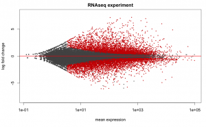
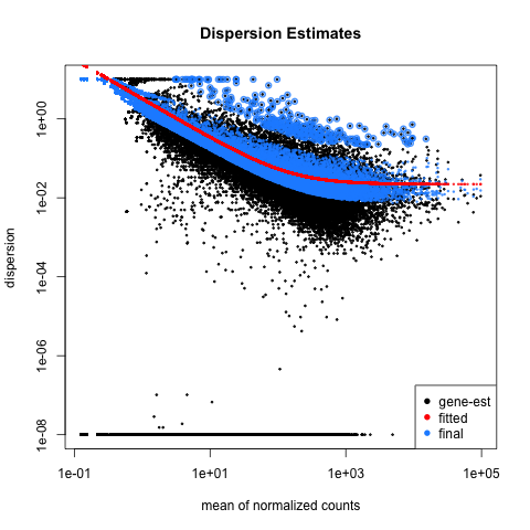
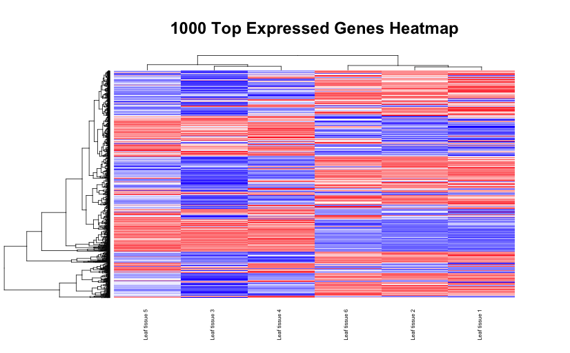
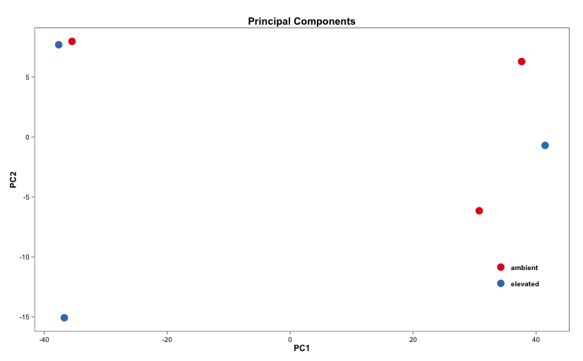
Below are some examples of the types of plots you can generate from RNAseq data using DESeq2:
Merging Data and Using Biomart:
To continue with analysis, we can use the .csv files we generated from the DeSEQ2 analysis and find gene ontology. This next script contains the actual biomaRt calls, and uses the .csv files to search through the Phytozome database. If you are trying to search through other datsets, simply replace the “useMart()” command with the dataset of your choice. Again, the biomaRt call is relatively simple, and this script is customizable in which values you want to use and retrieve.
# Install biomaRt package
source("http://bioconductor.org/biocLite.R")
biocLite("biomaRt")

# Load biomaRt library
library("biomaRt")

# Convert final results .csv file into .txt file
results_csv <- "Gmax_DESeq2-replaceoutliers-results.csv"
write.table(read.csv(results_csv), gsub(".csv",".txt",results_csv))
results_txt <- "Gmax_DESeq2-replaceoutliers-results.txt"

# List available biomaRt databases
# Then select a database to use
listMarts("phytozome_mart", host="phytozome.jgi.doe.gov",path="/biomart/martservice")
ensembl=useMart("phytozome_mart", host="phytozome.jgi.doe.gov", path="/biomart/martservice")

# List available datasets in database
# Then select dataset to use
listDatasets(ensembl)
ensembl = useMart("phytozome_mart", host="phytozome.jgi.doe.gov",path="/biomart/martservice", dataset="phytozome")

# Check the database for entries that match the IDs of the differentially expressed genes from the results file
a <- read.table(results_txt, head=TRUE)

b <- getBM(attributes=c('transcript_id',
 'chr_name1',
 'gene_name1',
 'gene_chrom_start',
 'gene_chrom_end',
 'kog_desc'),
 filters=c('pac_transcript_id'),
 values=a$X,
 mart=ensembl)
biomart_results <- "Gmax_DESeq2-Biomart.txt"
write.table(b,file=biomart_results)
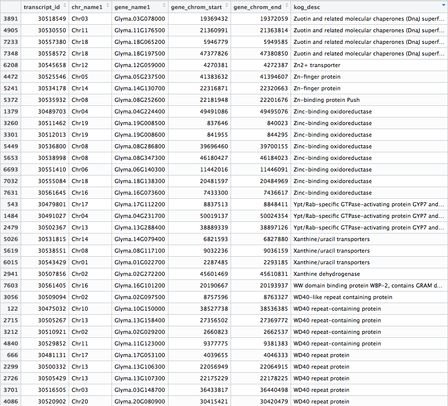
After fetching data from the Phytozome database based on the PAC transcript IDs of the genes in our samples, a .txt file is generated that should look something like this:
Finally, we want to merge the deseq2 and biomart output.
# Merge the deseq2 and biomart output
m <- merge(a, b, by="X")
write.csv(as.data.frame(m),file = "Gmax_DEseq2-Biomart-results_merged.csv")
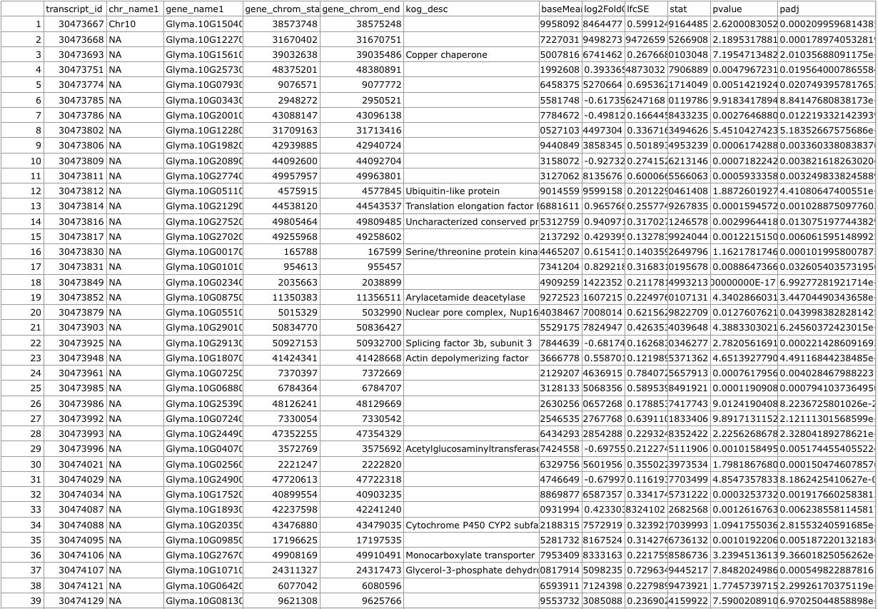
We get a merged .csv file with our original output from DESeq2 and the Biomart data:
Visualizing Differential Expression with IGV:
To visualize how genes are differently expressed between treatments, we can use the Broad Institute’s Interactive Genomics Viewer (IGV), which can be downloaded from here: IGV
We will be using the .bam files we created previously, as well as the reference genome file in order to view the genes in IGV. IGV requires that .bam files be indexed before being loaded into IGV. There is a script file located in
/common/RNASeq_Workshop/Soybean/STAR_HTSEQ_mapping/bam_files called bam_index.sh that will accomplish this. The .bam files themselves as well as all of their corresponding index files (.bai) are located here as well. The reference genome file is located at
/common/RNASeq_Workshop/Soybean/gmax_genome/Gmax_275_v2
You will need to download the .bam files, the .bai files, and the reference genome to your computer. Once you have IGV up and running, you can load the reference genome file by going to Genomes -> Load Genome From File… in the top menu. Now you can load each of your six .bam files onto IGV by going to File -> Load from File… in the top menu. Be sure that your .bam files are saved in the same folder as their corresponding index (.bai) files. Once you have everything loaded onto IGV, you should be able to zoom in and out and scroll around on the reference genome to see differentially expressed regions between our six samples.
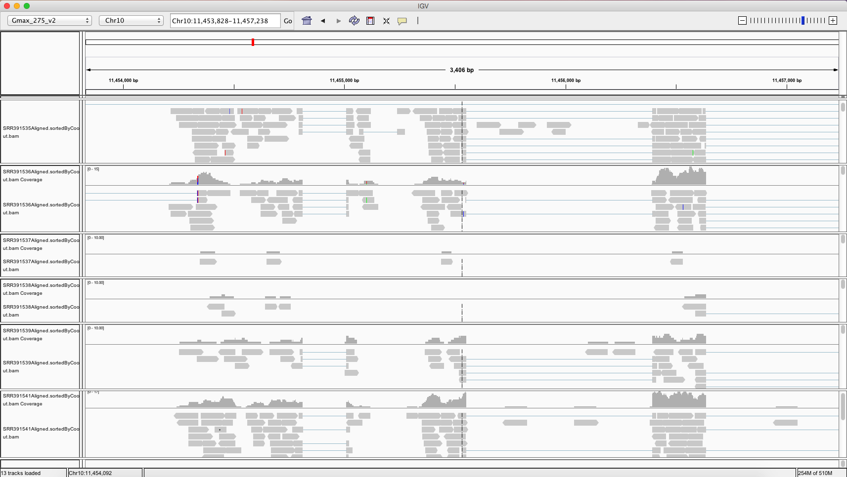
The differentially expressed gene shown is located on chromosome 10, starts at position 11,454,208, and codes for a transferrin receptor and related proteins containing the protease-associated (PA) domain. This information can be found on line 142 of our merged csv file. You can search this file for information on other differentially expressed genes that can be visualized in IGV!