How can K-mer estimation help to find genome sizes?
For a given sequence of length L, and a k-mer size of k, the total k-mer’s possible will be given by ( L – k ) + 1
e.g. In a sequence of length of 14, and a k-mer length of 8, the number of k-mer’s generated will be:
GATCCTACTGATGC ( L = 14 ) on decomposition of k-mers of length k = 8,

Total number of k-mer's generated will be
n = ( L - k ) + 1
  = (14 - 8 ) + 1
  = 7

GATCCTAC,     ATCCTACT,     TCCTACTG,     CCTACTGA,     CTACTGAT,     TACTGATG,     ACTGATGC
For shorter fragment sizes, as in the above example, the Total number of k-mers estimated is n = 7, and it is not close to actual fragment size of L which is 14 bps. But for larger fragment size, the total number of k-mer’s (n) provide a good approximation to the actual genome size. The following table tries to illustrate the approximation:
| k=18 | |||
|
Genome Sizes |
Total K-mers of k=18 |
% error in genome estimation |
|
| L | N=(L-K)+1 | ||
| 100 | 83 | 17 | |
| 1000 | 983 | 1.7 | |
| 10000 | 9983 | 0.17 | |
| 100000 | 99983 | 0.017 | |
| 1000000 | 999983 | 0.0017 | 1MB genome size |
So for a genome size of 1 Mb, the error between estimation and reality is only .0017%. Which is a very good approximation of actual size.
In the case of, 10 copies (C) of GATCCTACTGATGC sequence, then the total no of k-mer’s (n) of length k = 8 will be 70.
n      = [( L - k ) + 1 ] * C
       = [(14 - 8 ) + 1] * 10
       = 70
To get the actual genome size, we simply need to divide the total by the number of copies:
       = n / C
       = 70 / 10
       = 7
That will help us to understand, that we never sequence a single copy of genome but a population. Hence we end up sequencing C copies of genome. This is also referred as coverage in sequencing. To obtain actual genome size (N), divide the total k-mers (n) by coverage (C).
N = n / C
k-mer Distribution of a Typical Real World Genome
Major issue that is faced in a real world genome sequencing projects is a non-uniform coverage of genome. This can be accounted to technical and biological variables.
example: biased amplification of certain genomic regions during PCR (a step in preparation of sequencing libraries) and presence of repetitive sequences in genome.
k-mer size:
The size of k-mers should be large enough allowing the k-mer to map uniquely to the genome (a concept used in designing primer/oligo length for PCR). Too large k-mers leads to overuse of computational resources.
In the first step, k-mer frequency is calculated to determine the coverage of genome achieved during sequencing. There are software tools like Jellyfish that helps in finding the k-mer frequency in sequencing projects. The k-mer frequency follows a pseudo-normal distribution (actually it is a Poisson distribution) around the mean coverage in histogram of k-mer counts.
Once the k-mer frequencies are calculated a histogram is plotted to visualize the distribution and to calculate mean coverage.
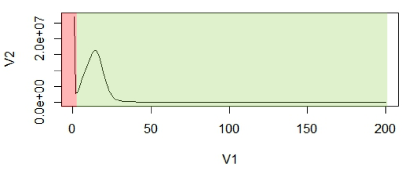
Figure 1: (A2) An example of k-mer histogram. The x-axis (V1), is the frequency or the number of times a given k-mer is observed in the sequencing data. The y-axis (V2), is the total number of k-mers with a given frequency.
The first peak is (in red region) primarily due to rare and random sequencing errors in reads. The values in graph can be trimmed to remove reads with sequencing errors.
With the assumption that k-mers are uniquely mapped to genome, they should be present only once in a genome sequence. So their frequency will reflect the coverage of the genome.
For calculation purposes we use mean coverage which is 14 in above graph. The area under the curve will represent the total number of k-mers.
So the genome estimation will be:
   N = Total no. of k-mers/Coverage
     = Area under curve /mean coverage(14)
Methodology
The study was conducted to estimate the genome size of the species with low coverage short read data to validate existing estimates (flow cytometry sourced) or produce a new computational estimate. The genome size is calculated from short sub-sequences (k-mers) of Illumina short read data. A larger k-mer size need to be considered for the genome estimation.
Reads should be quality controlled before the genome estimate is provided. Numerous programs exist for this purpose but Sickle (https://github.com/ucdavis-bioinformatics/sickle) is the application of choice in this tutorial. We require a minimum Phred-scaled quality value of 25 to for estimates.
Upon performing quality control, the k-mer distribution was calculated using the Jellyfish k-mer counting program. Then a histogram was constructed to perform the genome estimation using the same program.
The R statistical package is used to plot the binned distributions for the selected k-mer lengths. Initally the full data set is plotted and initial data points are often very high number due to the low frequency data points, and thus it should be avoided. Once the peak position is determined the total number of k-mers in the distribution is calculated, and then the genome size can be estimated using the peak position. In the ideal situation (or theoretically) the peak shape should be a Poisson distribution. In order to come up with a k-mer size a number of k-mer sizes are selected and genome estimation is done, where we see a regular distribution of the genome size.
Data sets used in this tutorial are available on BBC cluster:
Path: /common/Tutorial/Genome_estimation
Data sets: sample_read_1.fastq   sample_read_2.fastq
Script: GenomeEstimationScript.sh
Tutorial Outline
- Count k-mer occurrence using Jellyfish 2.2.6
- Generate histogram using R
- Determine the single copy region and the total k-mers
- Determine peak position and genome size
- Compare the peak shape with Poisson distribution
1. Count k-mer occurrence using Jellyfish 2.2.6
jellyfish count -t 8 -C -m 19 -s 5G -o 19mer_out --min-qual-char=? /common/Tutorial/Genome_estimation/sample_read_1.fastq /common/Tutorial/Genome_estimation/sample_read_2.fastq
options used in the counting k-mers:
-t    -treads=unit32       Number of treads to be used in the run. eg: 1,2,3,..etc.
-C    -both-strands        Count both strands
-m    -mer-len=unit32      Length of the k-mer
-s    -size=unit32         Hash size / memory allocation
-o    -output=string       Output file name
--min-quality-char         Base quality value. Version 2.2.3 of Jellyfish uses the “Phred” score, where "?" = 30
If you need to look at a detailed usage of ‘count’ in jellyfish, type the following after loading the jellyfish module.
jellyfish <cmd> [options]

jellyfish count --help
or
jellyfish count --full-help
In order to run the program Jellyfish in the bbc cluster, compose the following script and save it or you can copy GenomeEstimationScript.sh from the bbc cluster, which is located at the following path. (More on the commands used in the script can be found in here)
#!/bin/bash
#$ -N jellyfish
#$ -M user_email_id
#$ -q highmem.q
#$ -m bea
#$ -S /bin/bash
#$ -cwd
#$ -pe smp 8
#$ -o JellyFish_$JOB_ID.out
#$ -e Jellyfish_$JOB_ID.err

module load jellyfish/2.2.6
jellyfish count -t 8 -C -m 19 -s 5G -o 19mer_out --min-qual-char=? /common/Tutorial/Genome_estimation/sample_read_1.fastq /common/Tutorial/Genome_estimation/sample_read_2.fastq
It will create a out put file called 19mer_out. Then using the above created file (19mer_out), data points for a histogram will be created using the following command:
jellyfish histo -o 19mer_out.histo 19mer_out
If you open the 19mer_out.histo file, it will have the frequency counting of each k-mer with the k-mer length of 19.
1 13016694
2 3159677
3 3938273
4 5416130
5 7140173
6 8860956
7 10461902
8 11938782
9 13277372
10 14419501
11 15230762
12 15594907
13 15416499
14 14655690
15 13442589
16 11834646
17 10049240
18 8239408
19 6533641
20 5047445
21 3808930
22 2817665
23 2069050
24 1522365
25 1134562
2. Plot results using R
To visualize and to plot the data we use R Studio. Using the following command, we will load the data from the out_19mer.histo file in to a data frame called dataframe19.
dataframe19 <- read.table("19mer_out.histo") #load the data into dataframe19
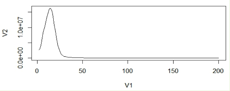
plot(dataframe19[1:200,], type="l") #plots the data points 1 through 200 in the dataframe19 using a line
This will create a line graph using the first 200 data points and the graph will look like the following:
In general, very low frequency k-mers represent high numbers that would skew the y –axis. If we look at the data points in the histogram file, we can see that the very first data point has a exceptionally high value than the next (second) data point. So we remove just the first line and re-plot using R. From now on we will disregard the first data point for our calculations.
plot(dataframe19[2:200,], type="l")
3. Determine the single copy region and the total number of k-mers
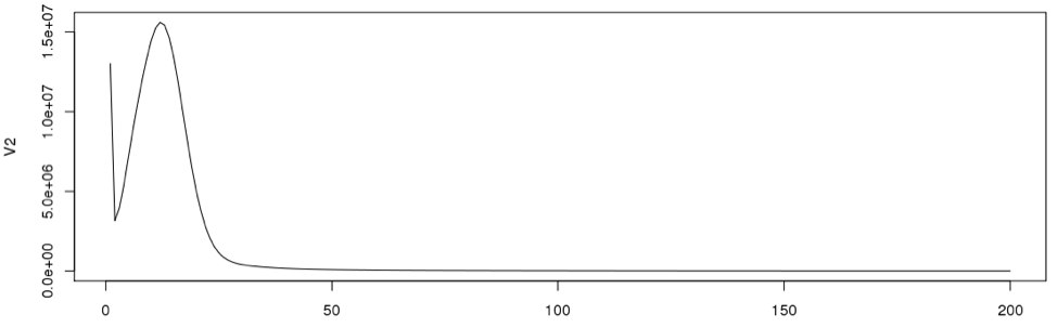
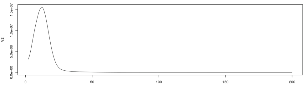
To determine the cut off points in the single copy region, we need to see the actual data point positions in the graph. In the initial examination the peak starts from the 2nd data point onward. So we will disregard the first data point in determining the single copy region.
Now using R we will re-plot the graph to determine the single copy region. Then we will include the points for clarity on the same graph.
plot(dataframe19[2:100,], type="l") #plot line graph
points(dataframe19[2:100,]) #plot the data points from 2 through 100
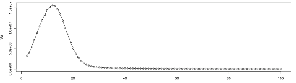
According to the graph, the single copy region would be between points 2 and 28.
Assuming the total number of data points is 9325, we can now calculate the total k-mers in the distribution.
sum(as.numeric(dataframe19[2:9325,1]*dataframe19[2:9325,2]))
It will produce the results as:
[1] 3667909811
4. Determine peak position and genome size
From the plotted graph we can get an idea where the peak position lies, and it should be between 5-20 data points. Now to determine the peak, thus, we need to look at the actual data points in that region. Using the below command we will examine the actual data points between 5 and 20.
data[10:20,]

    V1   V2

5   5 7140173
6   6 8860956
7   7 10461902
8   8 11938782
9   9 13277372
10 10 14419501
11 11 15230762
12 12 15594907
13 13 15416499
14 14 14655690
15 15 13442589
16 16 11834646
17 17 10049240
18 18 8239408
19 19 6533641
In this case the peak is at, 12. So the Genome Size can be estimated as:
sum(as.numeric(dataframe19[2:9325,1]*dataframe19[2:9325,2]))/12
Where the genome size is:
[1] 305659151
~ 305 Mb
It would be interesting to see the proportionality of the single copy region compared to the total genome size. In this data set the single copy region is between data point 2 and 28, So the size of single copy region can be roughly calculated as:
sum(as.numeric(dataframe19[2:28,1]*dataframe19[2:28,2]))/12
[1] 213956126
~ 213 Mb
The proportion can be calculated as:
(sum(as.numeric(dataframe19[2:28,1]*dataframe19[2:28,2]))) / (sum(as.numeric(dataframe19[2:9325,1]*dataframe19[2:9325,2])))
[1] 0.6999827
~ 70 %
5. Compare the peak shape with Poisson distribution
Since we have a nice curve, we can compare our curve to a theoretical curve, which is the Poission distribution.
singleC <- sum(as.numeric(dataframe19[2:28,1]*dataframe19[2:28,2]))/12
poisdtb <- dpois(1:100,12)*singleC
plot(poisdtb, type='l', lty=2, col="green")
lines(dataframe19[1:100,12] * singleC, type = "l", col=3)#, Ity=2)
lines(dataframe19[1:100,],type= "l")
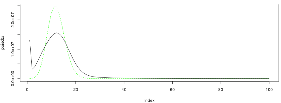
Likewise the procedure can be iterated across different number of k-mers.
| K-mer length | 19 | 21 | 23 | 25 | 27 | 29 | 31 |
| total No of fields | 9741 | 9653 | 9436 | 9325 | 9160 | 8939 | 8818 |
| Total K-mer count | 3.66E+09 | 4.4E+09 | 4.53E+09 | 4.67E+09 | 4.26E+09 | 4.44E+09 | 3.98E+09 |
| Genome size | 3.05E+08 | 2.9E+08 | 3.02E+08 | 3.14E+08 | 3.04E+08 | 3.41E+08 | 3.06E+08 |
| single copy region | 2.13E+08 | 2E+08 | 2.08E+08 | 2.25E+08 | 2.21E+08 | 2.36E+08 | 2.3E+08 |
| Proportion | 0.69998 | 0.69403 | 0.688915 | 0.716151 | 0.725814 | 0.690277 | 0.750801 |