This tutorial will introduce Single-cell RNA library preparation and provide guideline for single cell library analysis by using Cell Ranger. We will learn basics of Single Cell 3’ Protocol, and run Cell Ranger pipelines on a single library as demonstration. 

We will go through:

• Terminology
• Library Preperation
• Cellranger mkfastq
• Cellranger count
• Cllranger aggr
• Cellranger reanalyze

The sample data in this tutorial are listed below:

• cellranger-tiny-bcl-1.2.0
• cellranger-tiny-bcl-samplesheet-1.2.0.csv
• refdata-cellranger-GRCh38-1.2.0
• refdata-cellranger-hg19-1.2.0

 

Terminology

Throughout the documentation, you will see references to samples, libraries and sequencing runs. We define these as follows:

• Sample: A cell suspension extracted from a single biological source (blood, tissue, etc).
• Library: A 10x-barcoded sequencing library prepared from a single sample, corresponding to a single chip channel of a 10x Chromium Controller run.
• Sequencing Run / Flowcell: A flowcell containing data from one sequencing instrument run. The sequencing data can be further addressed by lane and by one or more sample indices.

The relationship between these terms can be complex:

• A single sample may be prepared into multiple libraries; this is commonly done to achieve higher cell counts without overloading a single 10x Chromium Controller run.
• A single library may be sequenced across multiple flowcells, and then combined as if all the reads came from one sequencing run.
• A single flowcell may contain multiple libraries, separated using different lanes and / or sample indices.
• The definition of “library” makes no distinction between two channels of the same physical 10x chip, versus the same channel of two different chips.

Library Preparation

Step 1 – GEM Generation & Barcoding

The Single Cell 3’ Protocol upgrades short read sequencers to deliver a scalable microfluidic platform for 3’ digital gene expression profiling of 500 – 10,000 individual cells per sample. The 10xTM GemCodeTM Technology samples a pool of ~ 750,000 barcodes to separately index each cell’s transcriptome. It does so by partitioning thousands of cells into nanoliter-scale Gel Bead-In-EMulsions (GEMs), where all generated cDNA share a common 10x Barcode. Libraries are generated and sequenced from the cDNA and the 10x Barcodes are used to associate individual reads back to the individual partitions.

To achieve single cell resolution, the cells are delivered at a limiting dilution, such that the majority (~90- 99%) of generated GEMs contains no cell, while the remainder largely contain a single cell.

Upon dissolution of the Single Cell 3’ Gel Bead in a GEM, primers containing (i) an Illumina R1 sequence (read 1 sequencing primer), (ii) a 16 bp 10x Barcode, (iii) a 10 bp randomer and (iv) a poly-dT primer sequence are released and mixed with cell lysate and Master Mix. Incubation of the GEMs then produces barcoded, full- length cDNA from poly-adenylated mRNA. After incubation, the GEMs are broken and the pooled fractions are recovered.

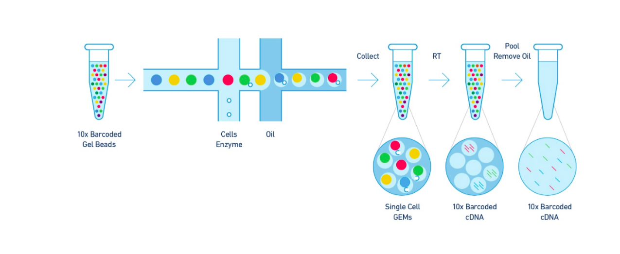
Step 2 – Post GEM-RT Cleanup & cDNA Amplification

Silane magnetic beads are used to remove leftover biochemical reagents and primers from the post GEM reaction mixture. Full-length, barcoded cDNA is then amplified by PCR to generate sufficient mass for library construction.

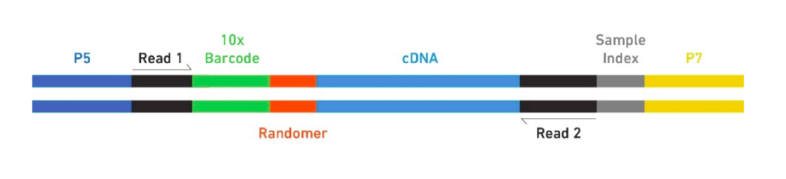
Step 3 – Library Construction

Enzymatic Fragmentation and Size Selection are used to optimize the cDNA amplicon size prior to library construction. R1 (read 1 primer sequence) are added to the molecules during GEM incubation. P5, P7, a sample index and R2 (read 2 primer sequence) are added during library construction via End Repair, A- tailing, Adaptor Ligation and PCR. The final libraries contain the P5 and P7 primers used in Illumina bridge amplification.

Step 4 – Sequencing Libraries

The Single Cell 3’ Protocol produces Illumina-ready sequencing libraries. A Single Cell 3’ Library comprises standard Illumina paired-end constructs which begin and end with P5 and P7. The Single Cell 3’ 16 bp 10xTM Barcode and 10 bp randomer is encoded in Read 1, while Read 2 is used to sequence the cDNA fragment. Sample index sequences are incorporated as the i7 index read. Read 1 and Read 2 are standard Illumina sequencing primer sites used in paired-end sequencing. The final structure of library are shown below, in which 10X barcode specifies cell and randomer specifies transcript. 

 

Library Analysis

Workflows

The Cell Ranger workflow always starts with running cellranger mkfastq on each flowcell. The subsequent steps vary depending on how many samples, libraries and flowcells you have. We will describe them in order of increasing complexity:

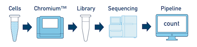
Single Sample, Library, and Flowcell is the most basic case. You have a single biological sample, which was prepared into a single library, and then sequenced on a single flowcell. Assuming the FASTQs have been generated with cellranger mkfastq, you just need to run cellranger count as described in Single-Library Analysis.

One Library, Multiple Flowcells If you have a library which was sequenced across multiple flowcells, you can pool the reads from both sequencing runs. Follow the steps in Multi-Flowcell Samples to combine them in a single cellranger count run.

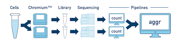
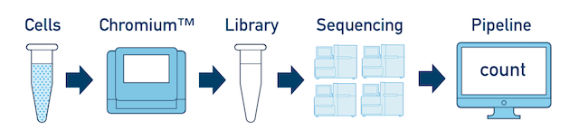
One Sample, Multiple Libraries If you prepared multiple libraries from the same sample (technical replicates, for example), then each one should be run through a separate instance of cellranger count. Once those are completed, you can perform a combined analysis using cellranger aggr, as described in Multi-Library Aggregation.

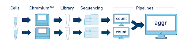
Multiple Biological Samples For a full experiment involving multiple biological samples, you must run cellranger count separately for each individual library deriving from each of those samples. For instance, if your experiment involves four samples, each having two libraries / replicates, then you will have to run cellranger count eight times. Then you can combine them all in a single call to cellranger aggr.

Cellranger mkfastq

The cellranger mkfastq pipeline is a 10x-enhanced wrapper around Illumina bcl2fastq, which demultiplexes BCL files from a sequencer into FASTQs for analysis. In this section, we uses the tiny-bcl example sequencing run as example. you don’t have to  download file to the working directory since the file is located at /common/RNASeq_Workshop/SingleCell/, but, for teaching purpose, download instruction for sample data are shown below:

wget http://cf.10xgenomics.com/supp/cell-exp/cellranger-tiny-bcl-1.2.0.tar.gz

The file is a zipped tar file. To unzip the file, type:

tar -xvzf cellranger-tiny-bcl-1.2.0.tar.gz

This will create a new subdirectory called cellranger-tiny-bcl-1.2.0. To run mkfastq pipeline, an Illumina Experiment Manager (IEM) sample sheet is also required. Note that his sample sheet is an example that is only valid for the Single Cell 3′ v2 chemistry.  enter command below to download the data sheet:

wget http://cf.10xgenomics.com/supp/cell-exp/cellranger-tiny-bcl-samplesheet-1.2.0.csv

Let’s briefly look at the tiny-bcl sample sheet before running the pipeline. It is a sample sheet that in the Illumina Experiment Manager (IEM) format. Note that you can specify a 10x sample index set in the index column of the Data section:

Here, SI-GA-C5 refers to a set of four separate sample indices. cellranger mkfastq also supports oligo sequences in the index column. In this example, only reads from lane 5 will be used. To search for the given sample index across all lanes, omit the lanes column entirely.

Before running the pipeline, we need to load cellrange by applying module load. You can check available version of Cellranger by typing module avail. In this example, we use CellRanger/1.2.1.

module load CellRanger/1.2.1

Next, we run Cellranger to generate FASTQs. Option --run specifies path to the unzipped BCL file you want to demultiplex. Option --samplesheet specifies path sample sheet, cellranger-tiny-bcl-samplesheet-1.2.0.csv in this case.This well take a few minutes. The shell script mkfastq.sh that runs the example can be found at /common/RNASeq_Workshop/SingleCell/.

cellranger mkfastq --run=/path/to/tiny_bcl \
                   --samplesheet=tiny-bcl-samplesheet.csv

Once the cellranger mkfastq pipeline has successfully completed, the output can be found in a new directory named with the serial number of the flowcell processed by cellranger mkfastq. The flowcell serial number for the tiny-bcl dataset is H77WWBBXX. The bcl2fastq output can be found in outs/fastq_path, and is organized in the same manner as a conventional bcl2fastq run.

In addition to generating FASTQs, the cellranger mkfastq pipeline writes both sequencing and 10x-specific quality control metrics into a JSON file. The metrics are in the outs/qc_summary.json file.There are quite a few metrics, but a few are particularly useful. Let’s look at the sample_qc key. To read entry associated with specific key, first open the JSON file with less:

less /common/RNASeq_Workshop/SingleCell/H35KCBCXY/outs/qc_summary.json

Then forward search the key by typing text below in less.

/sample_qc

This should return result as shown below. The sample_qc metric is a dictionary that contains one entry per distinct sample in the sample sheet, and one metrics structure per lane per sample, plus an ‘all’ structure in case a sample spans multiple lanes.

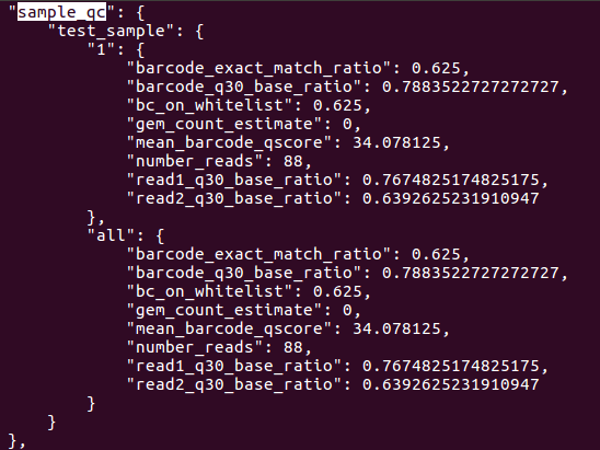
There are some other metrics we can check in order to diagnose low barcode mapping rates and read quality before running a cellranger pipeline. Keys and their functions are shown in chart below:
For a complete list of command-line arguments and additional information, run cellranger mkfastq --help.

Cellranger count

cellranger count takes FASTQ files from cellranger mkfastq and performs alignment, filtering, and UMI counting. It uses the Chromium cellular barcodes to generate gene-barcode matrices and perform clustering and gene expression analysis. count can take input from multiple sequencing runs on the same library.

We will use fastq files generated from previous section as sample data for this pipeline. In addition, we also need to download 2 transcriptome reference datasets and run cellranger twice in order to get 2 counts for aggr pipeline. Scripts for two runs are shown below. Both runs use refdata-cellranger-hg19-1.2.0. Shell script count.sh for this pipeline can be found at /common/RNASeq_Workshop/SingleCell.

cellranger count --id=sample1 --transcriptome=/common/RNASeq_Workshop/SingleCell/refdata-cellranger-hg19-1.2.0 --fastqs=/common/RNASeq_Workshop/SingleCell/H35KCBCXY/outs/fastq_path --sample=test_sample

cellranger count --id=sample2 --transcriptome=/common/RNASeq_Workshop/SingleCell/refdata-cellranger-hg19-1.2.0 --fastqs=/common/RNASeq_Workshop/SingleCell/H35KCBCXY/outs/fastq_path --sample=test_sample

As shown above, there are 4 required arguments. --id is a unique run ID string, which in the example is assigned arbitrarily as sample1 and sample2 respectively. --fastqs specifies path of the FASTQ directory generated by cellranger mkfastq. --sample indicates sample name as specified in the sample sheet supplied to mkfastq, which, in this case, can be found in cellranger-tiny-bcl-samplesheet-1.2.0.csv. --transcriptom specifies path to the Cell Ranger compatible transcriptome reference. For more optional arguments and additional information, enter cellranger count --help. The output of the pipeline will be contained in a diectory named with the sample ID you specified (e.g. sample345). The subdirectory named outs will contain the main pipeline output files. Detailed description of output is shown chart below:

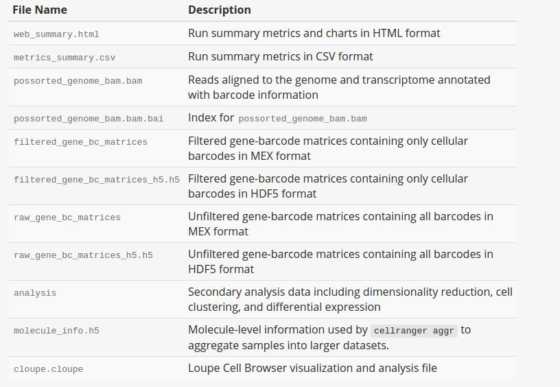
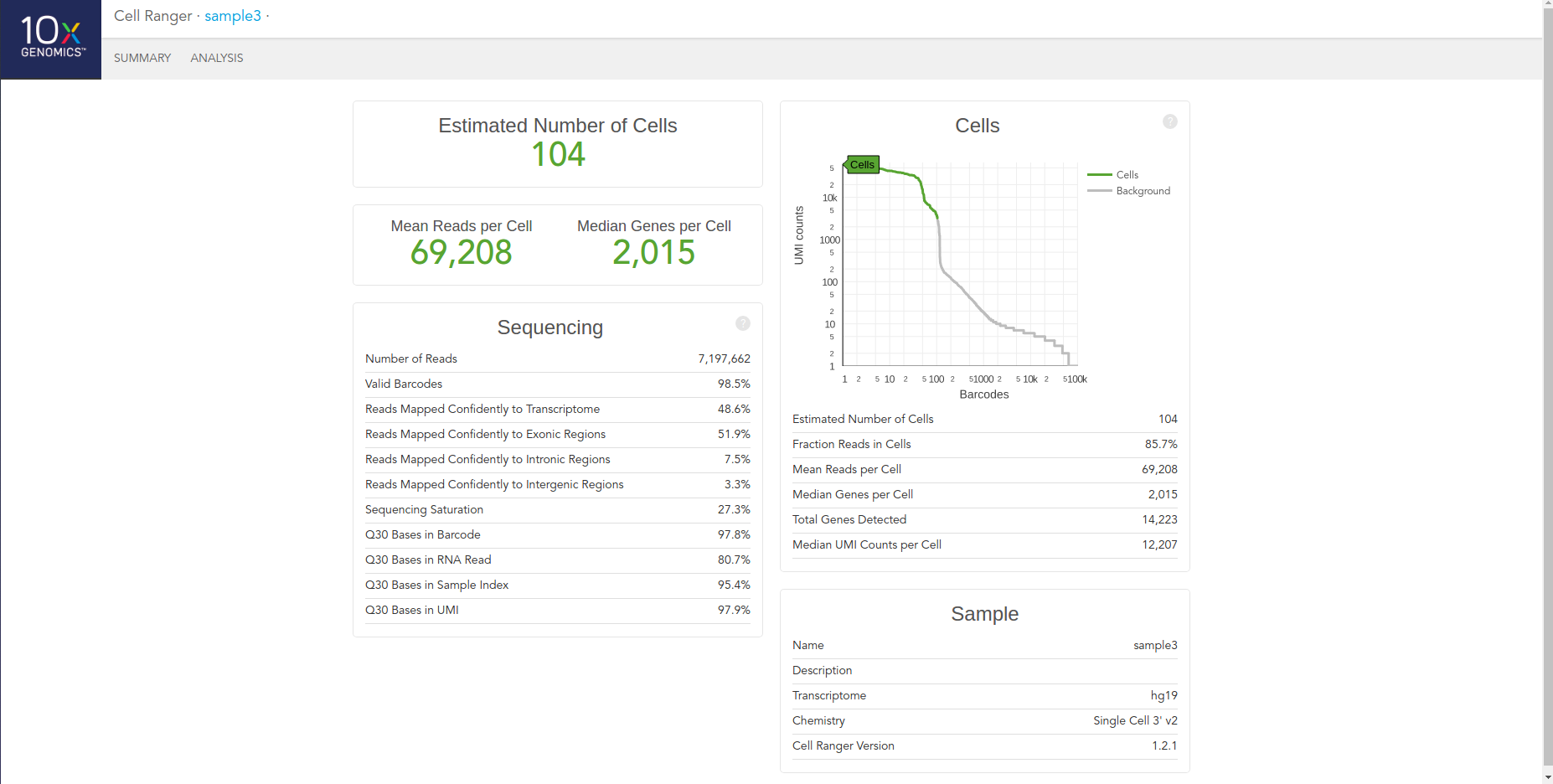
Once cellranger count has successfully completed, you can browse the resulting summary HTML file in any supported web browser, open the .cloupe file in Loupe Cell Browser, or refer to the Understanding Output section to explore the data by hand. Figure below shows results in html format.

Cellranger aggr
When doing large studies involving multiple biological samples (or multiple libraries / replicates of the same sample), it is best to run cellranger count on each of the libraries individually, and then pool the results using cellranger aggr. In this section, we use count data from previous section as example.

The cellranger aggr command takes a CSV file specifying a list of cellranger count output files (specifically the molecule_info.h5 from each run), and produces a single gene-barcode matrix containing all the data. The CSV file should contain 2 columns:

• library_id: Unique identifier for this input library. This will be used for labeling purposes only; it doesn’t need to match any previous ID you’ve assigned to the library. In our example, there are 2 library IDs, sample1 and sample2.
• molecule_h5: Path to the molecule_info.h5 file produced by cellranger count. In our case, 2 moluecule_info.h5 files are located in /sample1/outs/ and /sample2/outs/ repectively

We may create the CSV file either in a text editor or in Excel. Your CSV file should be similar to figure below.

The command shown below takes three arguments. --id is a unique run ID string specified by user. --csv is path to the CSV file that user creates. --normalize specifies how to normalize depth across the input libraries. This is an optional argument. The default value is mapped. The other two valid values are raw, and none. For details, see Depth Normalization. Both shell script aggr.sh and CSV file can be found at /common/RNASeq_Workshop/SingleCell/

cellranger aggr --id=AGG --csv=/common/RNASeq_Workshop/SingleCell/aggr.csv --normalize=mapped

Once cellranger has successfully completed, you can browse the resulting summary HTML file in any supported web browser, open the .cloupe file in Loupe Cell Browser, or refer to the Understanding Output section to explore the data by hand. For machine-readable versions of the summary metrics, refer to the cellranger aggr section of the Summary Metrics page.