/common/RNASeq_Workshop/MarineMarine/
|-- raw_data/
|-- quality_control/
|-- fastqc/
|-- index/
|-- mapping/
|-- counts/
|-- DESeq/
|-- entap/1. Accessing the Data using SRAtools
LF1A : SRR1964648, SRR1964649
LF2A : SRR1964647, SRR1964646
LB2A : SRR1964642, SRR1964643
LC2A : SRR1964644, SRR1964645
module load sratoolkit/2.8.1
 fastq-dump SRR1964642
 fastq-dump SRR1964643
/common/RNASeq_Workshop/Marine/raw_data/sratools.shraw_data/
|-- LB2A_SRR1964642.fastq
|-- LB2A_SRR1964643.fastq
|-- LC2A_SRR1964644.fastq
`-- LC2A_SRR1964645.fastqThe above folder is located at /common/RNASeq_Workshop/Marine/raw_data in BBC
2 Quality Control using Trimmomatic:
Trimmomatic performs quality control on illumina paired-end and single-end short read data. The following command can be applied to each of the four read fastq files:
java -jar /common/opt/bioinformatics/trimmomatic/0.36/trimmomatic-0.36.jar \
        SE \
        -threads 4 \
        /common/RNASeq_Workshop/Marine/raw_data/ \
        SLIDINGWINDOW:4:30 \
        MINLEN:50
Options:
SE                  Single end reads
-threads            number of processors
<input>             input file name
<output>            output file name
SLIDINGWINDOW:4:30  Scan the read with a 4-base wide sliding window, cutting when the average quality per base drops below 30
MINLEN:50           Removes any reads shorter than 50bp
/common/RNASeq_Workshop/Marine/quality_control/quality_control.shquality_control/
|-- quality_control.sh
|-- trim_LB2A_SRR1964642.fastq
|-- trim_LB2A_SRR1964643.fastq
|-- trim_LC2A_SRR1964644.fastq
`-- trim_LC2A_SRR1964645.fastqExamine the .out file generated during the run. It will provide a summary of the quality control process.
Input Reads: 26424138 Surviving: 21799606 (82.50%) Dropped: 4624532 (17.50%)3. FASTQC before and after QC
Create two directories: “before” and “after”.
module load fastqc/0.11.5
#looking at quality of the raw reads before doing trimming
fastqc --outdir ./before/ ../raw_data/LB2A_SRR1964642.fastq
This can be repeated for all you reads before trimming, which is your raw fastq files. The above script is located:/common/RNASeq_Workshop/Marine/fastqc/fastqc_before.sh
The same command can be used to look at the files after trimming.
module load fastqc/0.11.5
#looking at quality of the raw reads after doing trimming
fastqc --outdir ./after/ ../quality_control/trim_LB2A_SRR1964642.fastq.fastq
/common/RNASeq_Workshop/Marine/fastqc/fastqc_after.shOnce the analysis is done, it will produce a html file for each fastq file and a zip file which contains the images which have been used to illustrate in the html file. The final file structure will look as:
fastqc/
|-- after/
|   |-- trim_LB2A_SRR1964642_fastqc.html
|   |-- trim_LB2A_SRR1964642_fastqc.zip
|   |-- trim_LB2A_SRR1964643_fastqc.html
|   |-- trim_LB2A_SRR1964643_fastqc.zip
|   |-- trim_LC2A_SRR1964644_fastqc.html
|   |-- trim_LC2A_SRR1964644_fastqc.zip
|   |-- trim_LC2A_SRR1964645_fastqc.html
|   `-- trim_LC2A_SRR1964645_fastqc.zip
|-- before/
|   |-- LB2A_SRR1964642_fastqc.html
|   |-- LB2A_SRR1964642_fastqc.zip
|   |-- LB2A_SRR1964643_fastqc.html
|   |-- LB2A_SRR1964643_fastqc.zip
|   |-- LC2A_SRR1964644_fastqc.html
|   |-- LC2A_SRR1964644_fastqc.zip
|   |-- LC2A_SRR1964645_fastqc.html
|   `-- LC2A_SRR1964645_fastqc.zip
|-- fastqc_after.sh
`-- fastqc_before.sh
4. HISAT2: Aligning Single-End Short Reads to the Reference Genome
In order to map the reads to a reference genome, first you need to download the reference genome, and make a index file. We will be downloading the reference genome (https://www.ncbi.nlm.nih.gov/genome/12197) from the ncbi database, using the wget command.
wget ftp://ftp.ncbi.nlm.nih.gov/genomes/all/GCF/000/972/845/GCF_000972845.1_L_crocea_1.0/GCF_000972845.1_L_crocea_1.0_genomic.fna.gzThen we will use hisat2-build package in the software to make a HISAT index file for the genome. It will create a set of files with the suffix .ht2, these files together build the index, this is all you need to align the reads to the reference genome.
module load hisat2/2.0.5
hisat2-build -p 4 GCF_000972845.1_L_crocea_1.0_genomic.fna L_crocea
Usage: hisat2-build [options] <reference_in> <bt2_index_base>
reference_in comma-separated list of files with ref sequences
hisat2_index_base write ht2 data to files with this dir/basename
Options:
-p number of threads
/common/RNASeq_Workshop/Marine/index/hisat2_index.shL_croceaindex/
|-- GCF_000972845.1_L_crocea_1.0_genomic.fna
|-- hisat2_index.sh
|-- L_crocea.1.ht2
|-- L_crocea.2.ht2
|-- L_crocea.3.ht2
|-- L_crocea.4.ht2
|-- L_crocea.5.ht2
|-- L_crocea.6.ht2
|-- L_crocea.7.ht2
`-- L_crocea.8.ht2module load hisat2/2.0.5
hisat2 -p 4 --dta -x ../index/L_crocea -q ../quality_control/trim_LB2A_SRR1964642.fastq -S trim_LB2A_SRR1964642.samThe above need to be repeated for all the files.
Usage: hisat2 [options]* -x <ht2-idx>  [-S <sam>]
-x <ht2-idx>        path to the Index-filename-prefix (minus trailing .X.ht2)

Options:
-q                  query input files are FASTQ .fq/.fastq (default)
-p                  number threads
--dta               reports alignments tailored for transcript assemblers
The script is located at /common/RNASeq_Workshop/Marine/mapping/mapping.sh Once the mapping have been completed, the file structure is as follows:
mapping/
|-- mapping.sh
|-- trim_LB2A_SRR1964642.sam
|-- trim_LB2A_SRR1964643.sam
|-- trim_LC2A_SRR1964644.sam
`-- trim_LC2A_SRR1964645.sam
When HISAT2 completes its run, it will summarize each of it’s alignments, and it is written to the standard error file, which can be find in the same folder once the run is completed.
21799606 reads; of these:
  21799606 (100.00%) were unpaired; of these:
    1678851 (7.70%) aligned 0 times
    15828295 (72.61%) aligned exactly 1 time
    4292460 (19.69%) aligned >1 times
92.30% overall alignment ratesamtools view -@ 4 -uhS trim_LB2A_SRR1964642.sam | samtools sort -@ 4 - sort_trim_LB2A_SRR1964642
Usage: samtools [command] [options] in.sam
Command:
view     prints all alignments in the specified input alignment file (in SAM, BAM, or CRAM format) to standard output in SAM format

Options:
-h      Include the header in the output
-S      Indicate the input was in SAM format
-u      Output uncompressed BAM. This option saves time spent on compression/decompression and is thus preferred when the output is piped to another samtools command
-@      Number of processors

Usage: samtools [command] [-o out.bam]
Command:
sort    Sort alignments by leftmost coordinates

-o      Write the final sorted output to FILE, rather than to standard output.
The script for running all the samples is located at: /common/RNASeq_Workshop/Marine/mapping/sam2bam.sh Once the conversion is done you will have the following files in the directory.
mapping/
|-- sam2bam.sh
|-- sort_trim_LB2A_SRR1964642.bam
|-- sort_trim_LB2A_SRR1964643.bam
|-- sort_trim_LC2A_SRR1964644.bam
|-- sort_trim_LC2A_SRR1964645.bam
5 HTSEQ – Generating Total Read Counts from Alignments
htseq-count -s no -r pos -t gene -i Dbxref -f bam ../mapping/sort_trim_LB2A_SRR1964642.bam GCF_000972845.1_L_crocea_1.0_genomic.gff > LB2A_SRR1964642.counts
Usage: htseq-count [options] alignment_file gff_file
This script takes an alignment file in SAM/BAM format and a feature file in
GFF format and calculates for each feature the number of reads mapping to it.
See http://www-huber.embl.de/users/anders/HTSeq/doc/count.html for details.

Options:
  -f SAMTYPE, --format=SAMTYPE
                        type of  data, either 'sam' or 'bam'
                        (default: sam)
  -r ORDER, --order=ORDER
                        'pos' or 'name'. Sorting order of
                        (default: name). Paired-end sequencing data must be
                        sorted either by position or by read name, and the
                        sorting order must be specified. Ignored for single-
                        end data.
  -s STRANDED, --stranded=STRANDED
                        whether the data is from a strand-specific assay.
                        Specify 'yes', 'no', or 'reverse' (default: yes).
                        'reverse' means 'yes' with reversed strand
                        interpretation
  -t FEATURETYPE, --type=FEATURETYPE
                        feature type (3rd column in GFF file) to be used, all
                        features of other type are ignored (default, suitable
                        for Ensembl GTF files: exon)
  -i IDATTR, --idattr=IDATTR
                        GFF attribute to be used as feature ID (default,
                        suitable for Ensembl GTF files: gene_id)
/common/RNASeq_Workshop/Marine/counts/htseq.shcounts/
|-- htseq.sh
|-- sort_trim_LB2A_SRR1964642.counts
|-- sort_trim_LB2A_SRR1964643.counts
|-- sort_trim_LC2A_SRR1964644.counts
`-- sort_trim_LC2A_SRR1964645.counts
6 DESeq2 – Pairwise Differential Expression with Counts in R
# Marine DESeq Tutorial
# Download the DESeq2 try http:// if https:// URLs are not supported
source("https://bioconductor.org/biocLite.R")
biocLite("DESeq2")
# Load DESeq2 library
library("DESeq2")
# Set the working directory
directory <- "~/Documents/CBC/Tutorials/Marine/DESeq/two_sample_Control_Thermal_gene"
setwd(directory)
list.files(directory)
# Set the prefix for each output file name
outputPrefix <- "Croaker_DESeq2"
sampleFiles<- c("sort_trim_LB2A_SRR1964642.counts","sort_trim_LB2A_SRR1964643.counts",
"sort_trim_LC2A_SRR1964644.counts", "sort_trim_LC2A_SRR1964645.counts")
# Liver mRNA profiles of
# control group (LB2A), *
# thermal stress group (LC2A), *
sampleNames <- c("LB2A_1","LB2A_2","LC2A_1","LC2A_2")
sampleCondition <- c("control","control","treated","treated")
sampleTable <- data.frame(sampleName = sampleNames,
fileName = sampleFiles,
condition = sampleCondition)
ddsHTSeq <- DESeqDataSetFromHTSeqCount(sampleTable = sampleTable,
directory = directory,
design = ~ condition)
#By default, R will choose a reference level for factors based on alphabetical order.
# To chose the reference we can use: factor()
treatments <- c("control","treated")
ddsHTSeq$condition
#Setting the factor levels
colData(ddsHTSeq)$condition <- factor(colData(ddsHTSeq)$condition,
levels = treatments)
ddsHTSeq$condition
# Differential expression analysis
#differential expression analysis steps are wrapped into a single function, DESeq()
dds <- DESeq(ddsHTSeq)
# restuls talbe will be generated using results() which will include:
# log2 fold changes, p values and adjusted p values
res <- results(dds)
res
summary(res)
# filter results by p value
res= subset(res, padj<0.05)
# order results by padj value (most significant to least)
res <- res[order(res$padj),]
# should see DataFrame of baseMean, log2Foldchange, stat, pval, padj
# save data results and normalized reads to csv
resdata <- merge(as.data.frame(res),
as.data.frame(counts(dds,normalized =TRUE)),
by = 'row.names', sort = FALSE)
names(resdata)[1] <- 'gene'
write.csv(resdata, file = paste0(outputPrefix, "-results-with-normalized.csv"))
# send normalized counts to tab delimited file for GSEA, etc.
write.table(as.data.frame(counts(dds),normalized=T),
file = paste0(outputPrefix, "_normalized_counts.txt"), sep = '\t')
# produce DataFrame of results of statistical tests
mcols(res, use.names = T)
write.csv(as.data.frame(mcols(res, use.name = T)),
file = paste0(outputPrefix, "-test-conditions.csv"))
# replacing outlier value with estimated value as predicted by distrubution using
# "trimmed mean" approach. recommended if you have several replicates per treatment
# DESeq2 will automatically do this if you have 7 or more replicates
ddsClean <- replaceOutliersWithTrimmedMean(dds)
ddsClean <- DESeq(ddsClean)
temp_ddsClean <- ddsClean
tab <- table(initial = results(dds)$padj < 0.05,
cleaned = results(ddsClean)$padj < 0.05)
addmargins(tab)
write.csv(as.data.frame(tab),file = paste0(outputPrefix, "-replaceoutliers.csv"))
resClean <- results(ddsClean)
resClean = subset(res, padj<0.05)
resClean <- resClean[order(resClean$padj),]
write.csv(as.data.frame(resClean),file = paste0(outputPrefix, "-replaceoutliers-results.csv"))
####################################################################################
# Exploratory data analysis of RNAseq data with DESeq2
#
# these next R scripts are for a variety of visualization, QC and other plots to
# get a sense of what the RNAseq data looks like based on DESEq2 analysis
#
# 1) MA plot
# 2) rlog stabilization and variance stabiliazation
# 3) PCA plot
# 4) heatmap of clustering analysis
#
#
####################################################################################
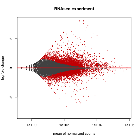
# MA plot of RNAseq data for entire dataset
# http://en.wikipedia.org/wiki/MA_plot
# genes with padj < 0.1 are colored Red
plotMA(dds, ylim=c(-8,8),main = "RNAseq experiment")
dev.copy(png, paste0(outputPrefix, "-MAplot_initial_analysis.png"))
dev.off()
# transform raw counts into normalized values
# DESeq2 has two options: 1) rlog transformed and 2) variance stabilization
# variance stabilization is very good for heatmaps, etc.
rld <- rlogTransformation(dds, blind=T)
vsd <- varianceStabilizingTransformation(dds, blind=T)
# save normalized values
write.table(as.data.frame(assay(rld),file = paste0(outputPrefix, "-rlog-transformed-counts.txt"), sep = '\t'))
write.table(as.data.frame(assay(vsd),file = paste0(outputPrefix, "-vst-transformed-counts.txt"), sep = '\t'))
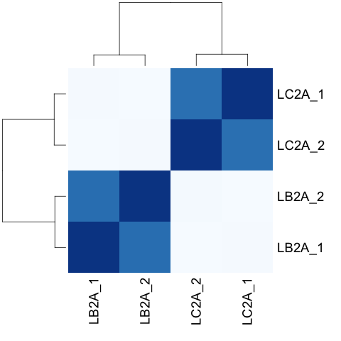
# clustering analysis
# excerpts from http://dwheelerau.com/2014/02/17/how-to-use-deseq2-to-analyse-rnaseq-data/
library("RColorBrewer")
library("gplots")
sampleDists <- dist(t(assay(rld)))
suppressMessages(library("RColorBrewer"))
sampleDistMatrix <- as.matrix(sampleDists)
rownames(sampleDistMatrix) <- paste(colnames(rld), rld$type, sep="")
colnames(sampleDistMatrix) <- paste(colnames(rld), rld$type, sep="")
colors <- colorRampPalette( rev(brewer.pal(8, "Blues")) )(255)
heatmap(sampleDistMatrix,col=colors,margin = c(8,8))
dev.copy(png,paste0(outputPrefix, "-clustering.png"))
dev.off()
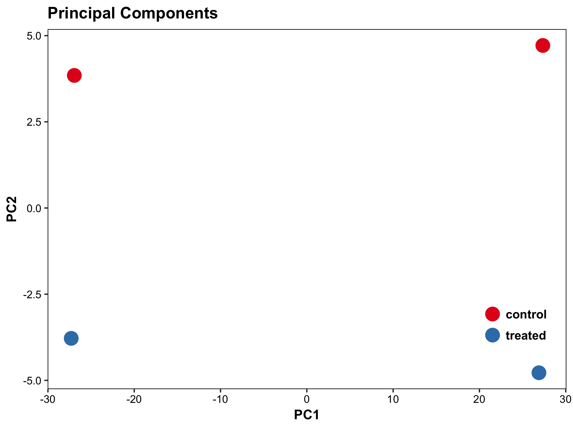
#Principal components plot shows additional but rough clustering of samples
library("genefilter")
library("ggplot2")
library("grDevices")
rv <- rowVars(assay(rld))
select <- order(rv, decreasing=T)[seq_len(min(500,length(rv)))]
pc <- prcomp(t(assay(vsd)[select,]))
# set condition
condition <- treatments
scores <- data.frame(pc$x, condition)
(pcaplot <- ggplot(scores, aes(x = PC1, y = PC2, col = (factor(condition))))
+ geom_point(size = 5)
+ ggtitle("Principal Components")
+ scale_colour_brewer(name = " ", palette = "Set1")
+ theme(
plot.title = element_text(face = 'bold'),
legend.position = c(.9,.2),
legend.key = element_rect(fill = 'NA'),
legend.text = element_text(size = 10, face = "bold"),
axis.text.y = element_text(colour = "Black"),
axis.text.x = element_text(colour = "Black"),
axis.title.x = element_text(face = "bold"),
axis.title.y = element_text(face = 'bold'),
panel.grid.major.x = element_blank(),
panel.grid.major.y = element_blank(),
panel.grid.minor.x = element_blank(),
panel.grid.minor.y = element_blank(),
panel.background = element_rect(color = 'black',fill = NA)
))
#dev.copy(png,paste0(outputPrefix, "-PCA.png"))
ggsave(pcaplot,file=paste0(outputPrefix, "-ggplot2.png"))
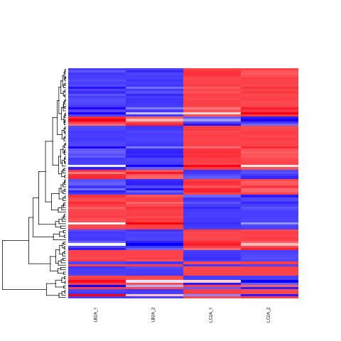
# heatmap of data
library("RColorBrewer")
library("gplots")
# 1000 top expressed genes with heatmap.2
select <- order(rowMeans(counts(ddsClean,normalized=T)),decreasing=T)[1:100]
my_palette <- colorRampPalette(c("blue",'white','red'))(n=100)
heatmap.2(assay(vsd)[select,], col=my_palette,
scale="row", key=T, keysize=1, symkey=T,
density.info="none", trace="none",
cexCol=0.6, labRow=F,
main="Heatmap of 100 DE Genes in Liver Tissue Comparison")
dev.copy(png, paste0(outputPrefix, "-HEATMAP.png"))
dev.off()
resulting files are located at: /common/RNASeq_Workshop/Marine/DESeq
7. EnTAP – Functional Annotation for DE Genes
Once the differentially expressed genes have been identified, we need to annotate the genes to identify the function. We will take the top 9 genes from the csv file to do a quick annotation. Will be useing the head command on the file, which will take the first 10 lines, and pipe it into a new file called temp.csv
head -n 10 Croaker_DESeq2-results-with-normalized.csv > temp.csv Then we are going to use a script which will link the geneID’s to the proteinID’s using the genome annotation in tabular format (ProteinTable12197_229515.txt) which can be downloaded from the NCBI website.
So the script will take the gene id’s from the temp.csv file and match it to the ProteinTable12197_229515.txt file and get the corresponding protein id’s. Then it will use that protein id to grab the fasta sequence from the protein fasta file.
python csvGeneID2fasta.py temp.csv ProteinTable12197_229515.txt GCF_000972845.1_L_crocea_1.0_protein.faa > GeneID_proteinID.txtUsage:
python csvGeneID2fasta.py [DE gene csv file] [tabular txt file] [fasta file]It will create a fasta file called “fasta_out.fasta” which will include the protein fasta sequences which we will be using for the enTAP job.
entap/
|-- Croaker_DESeq2-results-with-normalized.csv
|-- csvGeneID2fasta.py
|-- temp.csv
|-- GCF_000972845.1_L_crocea_1.0_protein.faa
|-- ProteinTable12197_229515.txt
|-- GeneID_proteinID.txt
`-- fasta_out.fasta
Once we have the fasta file with the protein sequences we can run the enTAP program to grab the functional annotations using the following command:
/tempdata3/alex/entap/enTAP/enTAP --runP -i fasta_out.fasta -d /common/Diamond/RefSeq/vertebrate_other.protein.faa.86.dmnd -d /common/Diamond/Uniprot-swiss/uniprot_sprot.dmnd --ontology 0 --threads 8
Required Flags:
--runP      with a protein input, frame selection will not be ran and annotation will be executed with protein sequences (blastp)
-i          Path to the transcriptome file (either nucleotide or protein)
-d          Specify up to 5 DIAMOND indexed (.dmnd) databases to run similarity search against

Optional:
-threads    Number of threads
--ontology  0 - EggNOG (default)
The script for the enTAP job is located at: /common/RNASeq_Workshop/Marine/entap/entap.sh
Once the job is done it will create a folder called “outfiles” which will contain the output of the program.
entap/
|-- outfiles/
|   |-- debug_2018.2.25-2h49m29s.txt
|   |-- entap_out/
|   |-- final_annotated.faa
|   |-- final_annotations_lvl0_contam.tsv
|   |-- final_annotations_lvl0_no_contam.tsv
|   |-- final_annotations_lvl0.tsv
|   |-- final_annotations_lvl3_contam.tsv
|   |-- final_annotations_lvl3_no_contam.tsv
|   |-- final_annotations_lvl3.tsv
|   |-- final_annotations_lvl4_contam.tsv
|   |-- final_annotations_lvl4_no_contam.tsv
|   |-- final_annotations_lvl4.tsv
|   |-- final_unannotated.faa
|   |-- final_unannotated.fnn
|   |-- log_file_2018.2.25-2h49m29s.txt
|   |-- ontology/
|   `-- similarity_search/
8. Integrating the DE Results with the Annotation Results
For this step you need to copy the following two files from the entap run to your computer, which is “GeneID_proteinID.txt” and “final_annotations_lvl0_contam.tsv” file from the previous run. The two files are located at,
entap/
|-- GeneID_proteinID.txt
|-- outfiles/
|   |-- final_annotations_lvl0_contam.tsv
Then we are going to integrate the annotations to the DE genes using the following R code:
library("readr")
#read the csv file with DE genes
csv <- read.csv("Croaker_DESeq2-results-with-normalized.csv")
#read the file with geneID to proteinID relationship
gene_protein_list <- read.table("GeneID_proteinID.txt")
names(gene_protein_list) <- c('GeneID','table', 'tableID','protein', 'protienID')
gene_protein_list <- gene_protein_list[,c("GeneID","protienID")]

#merging the two dataframes
DEgene_proteinID <- merge(csv, gene_protein_list, by.x="gene", by.y="GeneID")

#read_tsv
annotation_file <- read_tsv('final_annotations_lvl0.tsv', col_names = TRUE)
names(annotation_file)[1] <- 'query_seqID'

#merging the DEgene_proteinID with annotation_file dataframes
annotated_DEgenes <- merge(DEgene_proteinID, annotation_file, by.x="protienID", by.y="query_seqID")
View(annotated_DEgenes)
write.csv(annotated_DEgenes, file = paste0("annotated_DEgenes_final.csv"))