This tutorial will serve as a guideline for how to go about analyzing RNA sequencing data when a reference genome is available. We will go through alignment of the reads to the reference genome with HISAT2, conversion of the files to raw counts with stringtie and analysis of the counts with ballgown. The first two steps will be done on BBC server, while the last step will be performed on your local machine.
- Datasets Acquisition and Quality Control
- Mapping with HISAT2
- Transcript assembly and quantification with Stringtie
- Differential Expression Analysis with Ballgown
- Data visualization
The softwares and packages we’ll be using can be found here:
- SRAtoolkit(version 2.8.1/available on BBC)
- Sickle(available on BBC)
- fastqc(available on BBC)
- multiqc(available on BBC)
- HISAT2 (version 2.0.4/available on BBC)
- SAMtools (version 1.3.1/available on BBC)
- stringtie (version 1.3.0/available on BBC)
- R (version 3.3.1)
- ballgown (version 2.8.4)
The dataset we will use are single-end reads from a Ribosome profiling experiment. Four samples , isolated from rRNA, are selected. Among these 4 samples, two are from root tissues of Arabidopsis thaliana, while the others are from shoot tissues. They can be accessed from NCBI database with accession numbers: SRR3498212, SRR3498213, SRR3498215, SRR3498216. The reference genome of Arabidopsis thaliana used in this tutorial comes from JGI database. It is also stored in /common/Tutorial/Arabidopsis/
Datasets Acquisition and Quality Control
With accession number, we can download sample datasets by using sratoolkit. fastq-dump is command within sratoolkit allows user to download specific fastq file given its NCBI accession number.
fastq-dump SRR3498212
Repeat this command on sample SRR3498213, SRR3498215,and SRR3498216. Acquired raw fastq files and bash script SRAdump.sh are availble at /common/Tutorial/Arabidopsis/raw_data
Since SRA data is usually not quality controlled, we need to trim the data to eliminate short sequences and sequences with low qulity scores. Here we use sickle to do the job.
sickle se -f SRR3498212.fastq -t sanger -o trimmed_SRR3498212.fastq -q 35 -l 45
Flag se tell sickle the input file is single ended. -f indicates different input file -t indicates type of quality value. -o is the output file, -q is our minimum quality score and -l is the minimum read length. Repeat this command on sample SRR3498213, SRR3498215,and SRR3498216.
After trimming, we may use fastqc and multiqc to visualize the quality of data.
fastqc /common/Tutorial/Arabidopsis/raw_data/trimmed_SRR3498212.fastq
fastqc /common/Tutorial/Arabidopsis/raw_data/trimmed_SRR3498213.fastq
fastqc /common/Tutorial/Arabidopsis/raw_data/trimmed_SRR3498215.fastq
fastqc /common/Tutorial/Arabidopsis/raw_data/trimmed_SRR3498216.fastq

multiqc -f -n trimmed /common/Tutorial/Arabidopsis/raw_data/trimmed*
fastqc output quality control result to a html file. multiqc take html Quality Control run script and its output are stored in /common/Tutorial/Arabidopsis/raw_data.
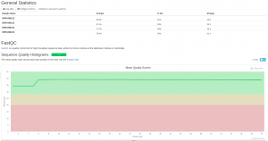
Mutiqc result before trimming
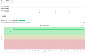
Multiqc result after trimming
Map the RNASeq reads to the genome
We use HISAT2 to alignment RNASeq reads to the reference genome. The mapping information allows us to collect subsets of the reads corresponding to each gene, and then to assemble and quantify transcripts represented by those reads. To use HISAT2, we first need to build reference with hisat2-build; function. This will generate a set of 6 files with suffixes .1.ht2, .2.ht2, .3.ht2, .4.ht2, .5.ht2, .6.ht2, .7.ht2. These files together constitute the index: they are all that is needed to align reads to that reference. The original sequence FASTA file downloaded from JGI database is no longer used by HISAT2 once the index is built.
hisat2-build -f /common/Tutorial/Arabidopsis/Athaliana_167_TAIR9.fa Athaliana
Here Athaliana_167_TAIR9.fa is A.Theliana reference genome downloaded from JGI database. Athaliana is the prefix assigned to output.
Run command below to align one of the reads from root tissues.
module load hisat2/2.0.5
hisat2 -p 8 --dta -x /common/Tutorial/Arabidopsis/index/Athaliana -q /common/Tutorial/Arabidopsis/trimmed_SRR3498212.fastq -S Athaliana_root_1.sam
-p: number of processors been used--dta: report alignments tailored for transcript assemblers-x: path to index generated from previous step-q: query input files in fastq format-S: output SAM file
Repeat this command on sample SRR3498213, SRR3498215, SRR3498216. Don’t forget to rename the output. To see detailed usage and all options, enter hisat2 -h in command line.
Before we move to next step, we need convert output SAM files to sorted BAM files, in order to fit requirement of Stringtie.
module load samtools/1.3.1
samtools sort -@ 4 -o Athaliana_root_1.bam /common/Tutorial/Arabidopsis/ReadAlignment/Athaliana_root_1.sam
-@: number of cores used-o: samtools output assigned by user
The shell scripts for mapping converting, as well as result SAM files and BAM file, are available at /common/Tutorial/Arabidopsis/.
Transcript assembly and quantification with StringTie
Analysis of RNA-seq experiments requires accurate reconstructions of all the isoforms expressed from each gene, as well as estimates of the relative abundance of those isoforms. Accurate quantification benefits from knowledge of precisely which reads originated from each isoform, which cannot be computed perfectly because reads are much shorter than transcripts. StringTie assembles transcripts from RNA-seq reads that have been aligned to the genome, first grouping the reads into distinct gene loci and then assembling each locus into as many isoforms as are needed to explain the data.
First, we need to convert GFF file downloaded from JGI database to GTF format. The command below will do the job.
gffread /common/Tutorial/Arabidopsis/Athaliana_167_TAIR10.gene.gff3 -T -o Athaliana_167_TAIR10.gene.gtf
An assembled gft file will be generated for each sample by using stringtie.
stringtie -p 8 -G /common/Tutorial/Arabidopsis/genes/Athaliana_167_TAIR10.gene.gtf -o Athaliana_root_1.gtf -l Athaliana /common/Tutorial/Arabidopsis/ReadAlignment/Athaliana_root_1.bam
-p: number of processors-G: Reference Genome downloaded from JGI database-o: output gtf file-l: SAM file mapped by HISAT2
Repeat this command for every sample. Enter stringtie -h to check more options.
The genes and isoforms present in one sample are rarely identical to those present in all other samples, but they need to be assembled in a consistent manner so that they can be compared, so we merge these GTF files into one single file. To accomplish that, we first need to make a document which serves as a index for stringtie to read. Create a txt file with vi, then enter files generated from the previous step, as shown below:
Athaliana_root_1.gtf
Athaliana_root_2.gtf
Athaliana_shoot_1.gtf
Athaliana_shoot_2.gtf
The command below takes the text file and returns a merged gtf file called stringtie_merged.gtf
stringtie --merge -p 8 -G /common/Tutorial/Arabidopsis/genes/Athaliana_167_TAIR10.gene.gtf -o stringtie_merged.gtf /common/Tutorial/Arabidopsis/genes/mergelist.txt
The script for assembly and merging, as well as the merge list, are available at /common/Tutorial/Arabidopsis/genes/.
Optionally, we can compare the new merged gtf file with the file we downloaded from the database, by running command below:
module load gffcompare/0.9.8
gffcompare –r /common/Tutorial/Arabidopsis/Athaliana_167_TAIR10.gene.gtf –G –o merged /common/Tutorial/Arabidopsis/genes/stringtie_merged.gtf
Finally, we use stringtie to generate count table for Ballgown analysis. Stringtie will compare each sample against merged assembly and estimate it transcript. abundance.
stringtie –e –B -p 8 -G /common/Tutorial/Arabidopsis/genes/stringtie_merged.gtf -o /common/Tutorial/Arabidopsis/ballgown/Athaliana_root_1/Athaliana_root_1.gtf /common/Tutorial/Arabidopsis/ReadAlignment/Athaliana_root_1.bam
-e: only estimate the abundance of given reference transcripts-B: enable output of Ballgown table files which will be created in the same directory as the output GTF-G: reference annotation generated from merging-o: path to the output countable specified by user
The command above takes a BAM file as input and generates a count table for ballgown. Repeat this step for other three samples. Note that it is important to arrange the output in hierarchy as shown below in order to let Ballgown automatically extract the data.
ballgown/
|-- Athaliana_root_1/
|   `-- Athaliana_root_1.gtf
|-- Athaliana_root_2/
|   `-- Athaliana_root_2.gtf
|-- Athaliana_shoot_1/
|   `-- Athaliana_shoot_1.gtf
`-- Athaliana_shoot_2/
    `-- Athaliana_shoot_2.gtf
The run script ballgown_prep.sh and output directory ballgown/ are save at /common/Tutorial/Arabidopsis/.
Download output directory ballgown/ to your local machine. Go to Unix Basics tutorial to learn how to transfer files to your local machine.
Differential Expression Analysis
The R programming language and the Bioconductor software suite host a comprehensive set of tools to handle tasks ranging from plotting raw data, to normalization, to downstream statistical modeling. In this tutorial, we use Ballgown package to analyze previously generated result. Ballgown, like other differential expression softwares, consisted of 4 major steps: (i) data visualization and inspection, (ii) statistical tests for differential expression, (iii) multiple test correction and (iv) downstream inspection and summarization of results. To setup Ballgown in your local machine, run following commands in your R console:
install.packages(″devtools″,repos=″http://cran.us.r-project.org″)
source(″http://www.bioconductor.org/biocLite.R″)
biocLite(c(″alyssafrazee/RSkittleBrewer″,″ballgown″, ″genefilter″,″dplyr″,″devtools″))
Note that Bioconductor version 3.0 or greater and R version 3.1 are required before installing ballgown.
The commands below will setup running environment by loading all required packages and working directory. The working directory you specified by user should contain the directory downloaded from BBC server.
library(ballgown)
library(RSkittleBrewer)
library(genefilter)
library(dplyr)
library(ggplot2)
library(gplots)
library(devtools)
dir <- "~/workspace/R/Arabidopsis" ##Define your own working directory accordingly
setwd(dir)
In addition to abundance data, Ballgown takes phenotype information as input. Phenotype data is supposed to be created by user and stored in csv format. Here, we divided our samples into two groups, root and shoot, based on their origin. You can create a csv file by yourself as shown below, or download phenodata.csv from BBC at /common/Tutorial/Arabidopsis/
| ids | part |
|---|---|
| Athaliana_root_1 | root |
| Athaliana_root_2 | root |
| Athaliana_shoot_1 | shoot |
| Athaliana_shoot_2 | shoot |
Then, we load phenodata.csv and phenodata.csv respectively:
pheno_data <- read.csv("phenodata.csv")
bg <- ballgown(dataDir = "ballgown", pData=pheno_data, samplePattern = "Athaliana")
In the second line, samplePattern specifies the common header in the name of each directory under ballgown.
Filter to remove low-abundance genes. One common issue with RNA-seq data is that genes often have very few or zero counts. A common step is to filter out some of these. Another approach that has been used for gene expression analysis is to apply a variance filter. Here we remove all transcripts with a variance across samples less than one:
bg_filt = subset(bg, "rowVars(texpr(bg))>1" ,genomesubset=TRUE)
To find transcripts that are deferentially expressed under variation. We use stattest function from Ballgown. We set getFC-TRUE so we that we can look at the confounder adjusted fold change between two groups.
results_transcripts = stattest(bg_filt, feature="transcript" , covariate = "part" , getFC = TRUE, meas = "FPKM")
Identify genes that show statistically significant differences between groups. For this we can run the same function that we used to identify differentially expressed transcripts, but here we set feature=”gene” in the stattest command:
results_genes = stattest(bg_filt, feature="gene" , covariate = "part" , getFC = TRUE, meas = "FPKM")
Add gene names and gene IDs to the results_transcripts data frame:
results_transcripts = data.frame(geneNames=ballgown::geneNames(bg_filt), geneIDs=ballgown::geneIDs(bg_filt), results_transcripts)
Sort the results from the smallest P value to the largest:
results_transcripts = arrange(results_transcripts,pval)
results_genes = arrange(results_genes,pval)
Write the results to a csv file that can be shared and distributed:
Identify transcripts and genes with a q value <0.05:
write.csv(results_transcripts, "transcript_results.csv", row.names=FALSE)
write.csv(results_genes, "gene_results.csv", row.names=FALSE)
Identify transcript and genes with a q-value < 0.05:
subset(results_transcripts,results_transcripts$qval<0.05)
subset(results_genes,results_genes$qval<0.05)
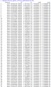
The result will pop up in console as shown below:
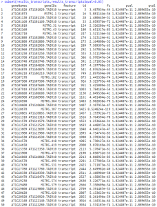
Transcripts with q-value < 0.5
Data Visualization
We use Ballgown to visualize RNA-seq results. The plots produced make it easier to compare between two groups.
We can obtain some nice colors and make plots pretty (Optional):
tropical = c('darkorange', 'dodgerblue', 'hotpink', 'limegreen', 'yellow')
palette(tropical)
Show the distribution of gene abundance measured as FPKM values across samples. The first command below extract the FPKM values. To transform FPKM values we use a log2 that adds one to all FPKM because log2(O) is undefined as shown in second line.
fpkm = texpr(bg, meas = "FPKM")
fpkm = log2(fpkm + 1)
boxplot(fpkm, col=as.numeric(pheno_data$part), las=2, ylab='log2(FPKM+1)')
We can make a plot of individual transcripts across samples. The first 2 commands show the name of the transcript and the name of the gene that contains it. The second 2 lines generate a box-and-whiskers plot, showing FPKM difference at that particular transcript. Here we use the 100th transcript as example.
ballgown::transcriptNames(bg)[100]
ballgown::geneNames(bg)[100]
plot(fpkm[100,] ~ pheno_data$part, border=c(1,2), main=paste(ballgown::geneNames(bg)[100], ' : ', ballgown::transcriptNames(bg)[100]), pch=19,
     xlab = "part", ylab='log2(FPKM+1)')
points(fpkm[100,] ~ jitter(as.numeric(pheno_data$part)), col=as.numeric(pheno_data$part))
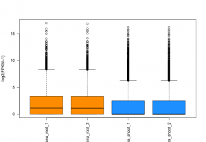
Distribution of FPKM values across the 4 samples. Sample from the same part of plant are labeled in the same color.
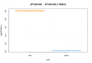
FPKM distribution in roots and shoots for transcript “AT1G01020”.
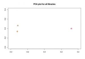
We can generate a PCA plot which shows correlation ‘distance’ between all libraries. Commands below identify the genes with a grand sum FPKM of at least 10 and calculate the correlation between all pairs of data. The correlations are converted to distance and coordiates by multi-dimensional scaling.
short_names = c("r1","r2","s1","s2")
i = which(apply(fpkm, 1, sum) > 10)
r = cor(fpkm[i, c(0:4)], use="pairwise.complete.obs",method="pearson")
d = 1 - r
mds=cmdscale(d, k=2, eig=TRUE)
par(mforw=c(1,1))
plot(mds$points, type="n", xlab="", ylab="", main="PCA plot for all libraries", xlim=c(-0.4,0.4), ylim=c(-0.4,0.4))
points(mds$points[,1], mds$points[,2],col="grey", cex=2, pch=16)
text(mds$points[,1], mds$points[,2],short_names, col=c(darkorange, darkorange, hotpink, hotpink))<\pre>
Reference
Hsu PY, Calviello L, Wu HL, Li FW et al. Super-resolution ribosome profiling reveals unannotated translation events in Arabidopsis. Proc Natl Acad Sci U S A 2016 Oct 21. PMID: 27791167
